Electricity production forecasting using ARIMA model in Python

Last Updated on February 19, 2021 by Editorial Team

Author(s): Jayashree domala

Data Visualization

Electricity Production Forecasting Using Arima Model in Python

A guide to the step-by-step implementation of ARIMA models using Python.

ARIMA which is the short form for ‘Auto-Regressive Integrated Moving Average’ is used on time series data and it gives insights on the past values like lags and forecast errors that can be used for forecasting future values.

To know more about ARIMA models, check out the article below:

A brief introduction to ARIMA models for time series forecasting

How to implement ARIMA models to help forecasting/predicting?

The steps involved are as follows:

1. Analyzing the time series data by plotting or visualizing it.
2. Converting the time series data in a stationary form.
3. Plotting the ACF and PACF plots.
4. Constructing the ARIMA model.
5. Making predictions using the model created.

Implementation using Python

→ Import packages

The basic packages like NumPy and pandas for dealing with data are imported. For visualization, matplotlib is used. And to implement the ARIMA model, the statsmodel is imported.

>>> import numpy as np
>>> import pandas as pd
>>> import statsmodels.api as sm
>>> import matplotlib.pyplot as plt
>>> %matplotlib inline

→ Analyzing data

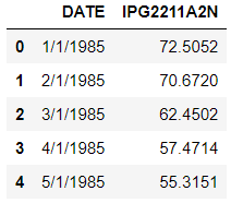
The data which is used is seasonal data of electricity production.

>>> df = pd.read_csv('Electric_Production.csv')
>>> df.head()

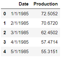
The column names are changed for ease of use.

>>> df.columns = ['Date','Production']
>>> df.head()

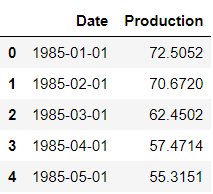
Now to work with time-series data, the ‘date’ column is converted into DateTime index.

>>> df['Date'] = pd.to_datetime(df['Date'])
>>> df.head()

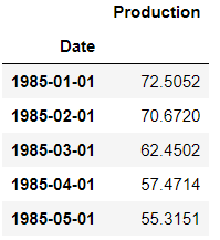
>>> df.set_index('Date',inplace=True)
>>> df.head()

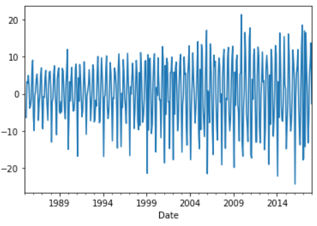
→ Visualization of data

>>> df.plot()

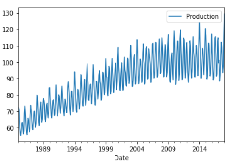
As seen from the plot, this is seasonal data as there is some seasonality to it and an upward trend too.

Now comparing the 12-month simple moving average along with the series to ascertain the trend. The standard deviation is also plotted to see if there is any variance or no.

>>> df['Production'].rolling(12).mean().plot(label='12 SMA',figsize=(16,8))
>>> df['Production'].rolling(12).std().plot(label='12 STD')
>>> df['Production'].plot()
>>> plt.legend()

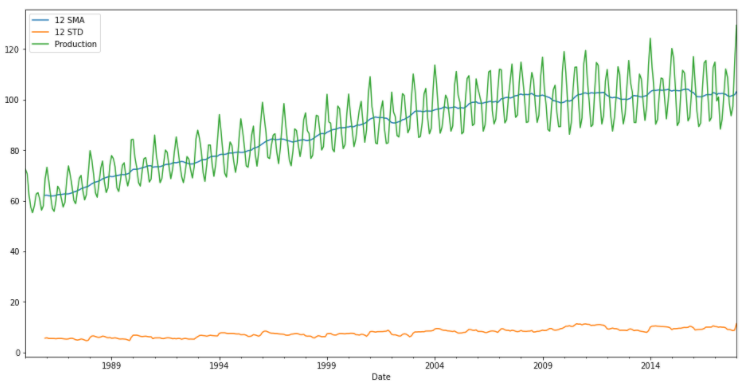
As seen from the above plot, the standard deviation is not varying much so there is not much variance.

→ Decomposition of the time series data to its trend, seasonality and residual components.

statsmodels is used for the decomposition.

>>> from statsmodels.tsa.seasonal import seasonal_decompose

>>> decomp = seasonal_decompose(df['Production'])
>>> fig = decomp.plot()
>>> fig.set_size_inches(14,7)

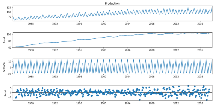
The trend, seasonal and residual errors can be seen individually here.

→ Converting the data into the stationary form

The data is first tested using the Dickey-Fuller test to check if the data is in stationary form or no and then change its form.

The Dickey-Fuller has the null hypothesis that a unit root is present and it is a non-stationary time series. The alternative hypothesis is that there is no unit root and the series is stationary.

We will test with the help of the parameter ‘p’. If p is small (p<=0.05), we reject the null hypothesis, otherwise not reject the null hypothesis.

From the statsmodels package, the augmented dickey-fuller test function is imported. It returns a tuple that consists of the values: adf, pvalue, usedlag, nobs, critical values, icbest and resstore.

>>> from statsmodels.tsa.stattools import adfuller

Then this function is called on the production column of the dataset.

>>> fuller_test = adfuller(df['Production'])
>>> fuller_test

(-2.256990350047239,
 0.18621469116586975,
 15,
 381,
 {'1%': -3.4476305904172904,
  '5%': -2.869155980820355,
  '10%': -2.570827146203181},
 1840.8474501627156)

Now the p-value is printed and using the p-value, it is ascertained if data is stationary or not.

>>> def test_p_value(data):
        fuller_test = adfuller(data)
        print('P-value: ',fuller_test[1])
        if fuller_test[1] <= 0.05:
            print('Reject null hypothesis, data is stationary')
        else:
            print('Do not reject null hypothesis, data is not stationary')

>>> test_p_value(df['Production'])

P-value:  0.18621469116586975
Do not reject null hypothesis, data is not stationary

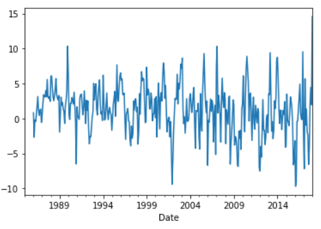
Since the data is not stationary, differencing is carried out. The difference is the change of the time series from one period to the next. The first difference, second difference and seasonal difference are calculated and for each, the p-value is checked.

df['First_diff'] = df['Production'] - df['Production'].shift(1)
df['First_diff'].plot()

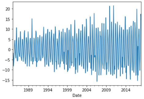
>>> test_p_value(df['First_diff'].dropna())

P-value:  4.0777865655398996e-10
Reject null hypothesis, data is stationary

In the first difference, we got the data in the stationary form. In case, a second difference was needed then the following would have been done.

>>> df['Second_diff'] = df['First_diff'] - df['First_diff'].shift(1)
>>> df['Second_diff'].plot()

>>> test_p_value(df['Second_diff'].dropna())

P-value:  4.1836937480000375e-17
Reject null hypothesis, data is stationary

A seasonal difference can also be taken as follows. The shifting will happen by an entire season that is ‘12’.

>>> df['Seasonal_diff'] = df['Production'] - df['Production'].shift(12)
>>> df['Seasonal_diff'].plot()

>>> test_p_value(df['Seasonal_diff'].dropna())

P-value:  8.812644938089026e-07
Reject null hypothesis, data is stationary

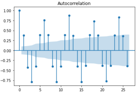
→ Plotting the ACF and PACF plot

From the statsmodels package, the ACF and PACF plot functions are imported.

>>> from statsmodels.graphics.tsaplots import plot_acf, plot_pacf

>>> first_diff = plot_acf(df['First_diff'].dropna())

>>> sec_diff = plot_pacf(df['Second_diff'].dropna())

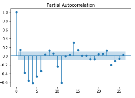
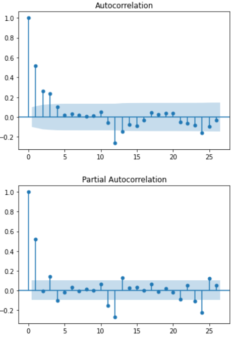
Now the final ACF and PACF plots will be plotted which will be used further.

>>> p1 = plot_acf(df['Seasonal_diff'].dropna())
>>> p2 = plot_pacf(df['Seasonal_diff'].dropna())

→ Constructing the ARIMA model

For non-seasonal data, the ARIMA model can be imported from statsmodels module.

>>> from statsmodels.tsa.arima_model import ARIMA

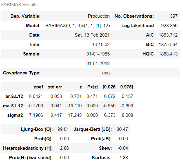
For seasonal data, the seasonal ARIMA model can be imported from the statsmodels module. The data used here is seasonal data so the seasonal ARIMA model is imported. The arguments passed are production column, order and seasonal order.

order: The (p,d,q) order of the model for the number of AR parameters, differences, and MA parameters.

seasonal order: The (P,D,Q,s) order of the seasonal component of the model for the AR parameters, differences, MA parameters, and periodicity.

>>> model = sm.tsa.statespace.SARIMAX(df['Production'],order=(0,1,0),seasonal_order=(1,1,1,12))

Once the model is created, the next thing to do is to fit the model.

>>> results = model.fit()
>>> results.summary()

To know about the residuals values or error, the ‘resid’ method can be called on the results.

>>> results.resid

Date
1985-01-01    72.505200
1985-02-01    -1.833200
1985-03-01    -8.221800
1985-04-01    -4.978800
1985-05-01    -2.156300
                ...    
2017-09-01     0.529985
2017-10-01     4.057874
2017-11-01     0.690663
2017-12-01     2.477697
2018-01-01     6.953533
Length: 397, dtype: float64

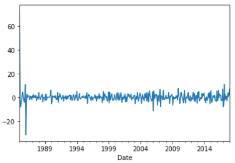
The plot of the residual points can be created.

>>> results.resid.plot()

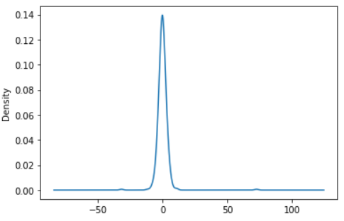
The distribution of the errors can be seen by plotting the KDE. And as seen from the plot below, the errors are distributed around 0 which is good.

>>> results.resid.plot(kind='kde')

→ Predicting or forecasting

By predicting the values, the model’s performance can be ascertained. First, we can look into how it predicts the data present and then move onto predicting future data.

>>> df['prediction'] = results.predict()
>>> df[['Production','prediction']].plot(figsize=(12,8))

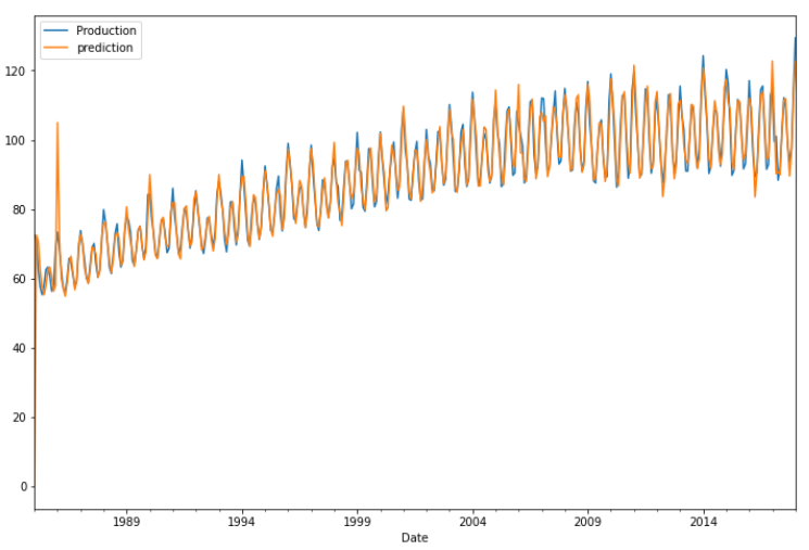
As seen from the above plot, the model does a good job is predicting the present data. Now to predict for the future, we can add more months to the dataset with null values and predict for it. This can be done using pandas. The last index is obtained which is the last date and a month offset is added to it which starts from 1 and goes up to 24.

>>> from pandas.tseries.offsets import DateOffset
>>> extra_dates = [df.index[-1] + DateOffset(months=m) for m in range (1,24)]

>>> extra_dates
[Timestamp('2018-02-01 00:00:00'),
 Timestamp('2018-03-01 00:00:00'),
 Timestamp('2018-04-01 00:00:00'),
 Timestamp('2018-05-01 00:00:00'),
 Timestamp('2018-06-01 00:00:00'),
 Timestamp('2018-07-01 00:00:00'),
 Timestamp('2018-08-01 00:00:00'),
 Timestamp('2018-09-01 00:00:00'),
 Timestamp('2018-10-01 00:00:00'),
 Timestamp('2018-11-01 00:00:00'),
 Timestamp('2018-12-01 00:00:00'),
 Timestamp('2019-01-01 00:00:00'),
 Timestamp('2019-02-01 00:00:00'),
 Timestamp('2019-03-01 00:00:00'),
 Timestamp('2019-04-01 00:00:00'),
 Timestamp('2019-05-01 00:00:00'),
 Timestamp('2019-06-01 00:00:00'),
 Timestamp('2019-07-01 00:00:00'),
 Timestamp('2019-08-01 00:00:00'),
 Timestamp('2019-09-01 00:00:00'),
 Timestamp('2019-10-01 00:00:00'),
 Timestamp('2019-11-01 00:00:00'),
 Timestamp('2019-12-01 00:00:00')]

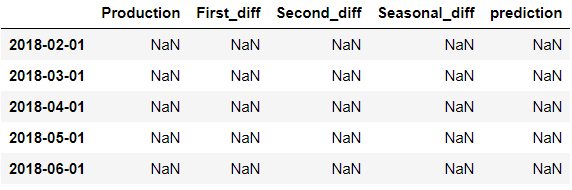
Now another dataframe is created with these extra future date values as an index and the rest of the column values as null.

>>> forecast_df = pd.DataFrame(index=extra_dates,columns=df.columns)
>>> forecast_df.head()

Now the original dataframe and this forecast dataframe are concatenated into a single one for forecasting.

>>> final_df = pd.concat([df,forecast_df])

Now we can predict the values for the end data points by mentioning the start and end arguments while calling the ‘predict’ function.

>>> final_df['prediction'] = results.predict(start=396, end=430)
>>> final_df[['Production','prediction']].plot(figsize=(12,8))

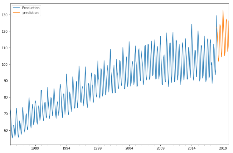
The prediction line can be seen clearly for the future values.

Conclusion

ARIMA model was successfully used to predict the future values for the electricity production which is a seasonal dataset with non-stationary behavior. Using the proper steps, the data was converted to the stationary form and the prediction model was built.

Refer to the notebook and dataset here.

Reach out to me: LinkedIn

Check out my other work: GitHub

---

Electricity production forecasting using ARIMA model in Python was originally published in Towards AI on Medium, where people are continuing the conversation by highlighting and responding to this story.

Published via Towards AI