Data Science Case Study — Credit Default Prediction: Part 2

Author(s): Saankhya Mondal

Originally published on Towards AI.

In financial institutions, credit default occurs when a borrower fails to fulfill their debt obligations, leading to a breach of the loan agreement. It represents the risk that a borrower will default on their debt, impacting lenders and investors. Machine learning models are increasingly being used for the predictive modeling of credit default.

In Part 1 of Data Science Case Study — Credit Default Prediction, we have talked about feature engineering, model training, model evaluation and classification threshold selection. This article is the continuation of Part 1. If you haven’t read Part 1, click here. Part 2 will discuss model explainability and how concepts borrowed from game theory, like Shapley values, will help us better understand the predictions of our model.

Let’s jump in!

Model Explainability

Our model can make predictions by feeding into it the features. Let’s suppose the model predicts that a customer will not default on the credit/loan. The financial institution wants to understand why the model is predicting what it is predicting. They want to understand why the customer be allowed the loan. Alternatively, if the model predicts that a customer will default on the loan if it is given, the bank/company would want to provide their customer with valid reasons why they can’t provide a loan. Additionally, they would like to provide customers with financial advice on how to improve their financial behavior to be reconsidered for loans.

This is where model explainability comes into picture. Our model is a black box, and we can uncover it by using techniques from Explainable AI. Researchers have come up with SHAP — a model explainability and interpretability technique using Shapley Values, a concept widely used in Game Theory.

What are Game Theory, cooperative games, and Shapley Values?

Game Theory is the study of mathematical models to understand the strategic behavior of and interactions between rational players in a competitive or cooperative setting. The setting is referred to as a “Game”. There are mainly two branches in Game Theory — non-co-operative and co-operative games. You may have heard of zero-sum games (recall ‘Generator’ vs ‘Discriminator’ in GANs) or Nash equilibrium, which is a part of non-cooperative game theory. Co-operative games involve players forming coalitions to achieve mutual goals, with outcomes shared among coalition members. Shapley values assign a value to each player, reflecting their marginal contribution to all possible coalitions, providing a fair and interpretable measure of individual importance or impact within a cooperative setting.

SHAP (Shapley Additive Explanations)

SHAP (Shapley Additive Explanations) is a model explainability technique based on Shapley values. Let’s suppose model prediction is a game. The feature involved are the players. They form a coalition. The model is a coalition of features. SHAP assigns each feature an importance value for a particular prediction.

The mathematical expression for Shapley values in the context of ML involves calculating the marginal contribution of each feature across different subsets of features. This is done by comparing the model’s output when a specific feature is included with the output when that feature is excluded.

Suppose n = {1, 2, 3, 4} represents four features. We want to calculate the Shapley value for feature 1.

1. We iterate through all possible subsets of n that don’t contain feature 1. These are S= {2}, S= {3}, S= {4}, S= {2, 3}, S= {2, 4}, S= {3, 4}, and S= {2, 3, 4}.
2. For each subset S, we compute the marginal contribution of feature 1 by comparing model’s prediction with actual value of feature 1 (included), f(S U {1}) and a random value of feature 1 (excluding or treating the feature 1 as noise), f(S).
3. |f(S U {1})-f(S)| represents the marginal contribution.
4. The final Shapley value for the feature 1 is computed by performing weighted sum of all the marginal contributions. The weight is probability of getting the subset of features, S among all the subsets.

You can refer this article for in-depth understanding of Shapley Values. Using SHAP, we can understand which feature has more importance or impact. Let’s see SHAP in action.

SHAP Summary Plot

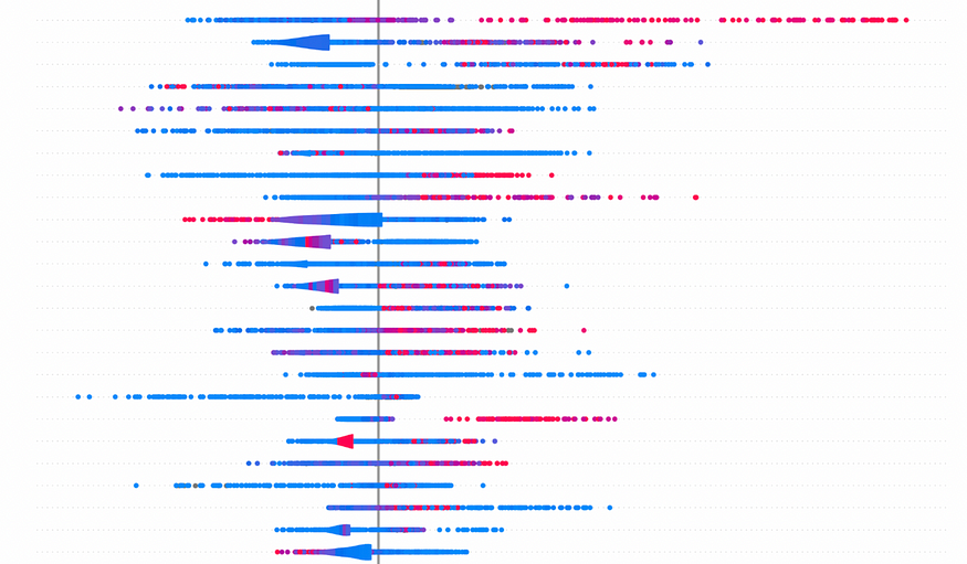
SHAP Summary Plot as the name suggest provides us a summary of the most important features and their SHAP value distributions. Each point on the plot is a SHAP Value. Color red represents higher value of the feature and color blue represents lower value of the feature. Consider the feature — count_casa_accounts. Higher value of this feature tends to have a higher Shapley Value and hence a more say in the model score. You can observe similar behavior for the feature num_loan_payments_missed_last_360_days.

SHAP Force and Decision Plot

SHAP Summary Plot shows us an aggregated picture. SHAP Force Plot helps us understand a single prediction by the model and provide explanations as to which feature impacts which score. SHAP Decision Plot describes the same but in a compact manner.

Consider two cases. The first case is the prediction for a customer who doesn’t default.

1. The model score is 0.13 whereas the base score (the average score of the model on the training data) is 0.1705. This is the score we get when we don’t have any features.
2. The feature in blue such as num_loan_accounts_lifetime forces the model score to reduce. num_loan_accounts_lifetime for this case is 2 whereas the average is 3. This tells that this customer has lesser loan number of loan accounts than the average, and hence the positive impact.
3. The feature in red such as last_closing_balance_amount_salary_month forces the model score to increase. last_closing_balance_amount_salary_month for this case is only 1232.76 whereas the average is 20345.61. This tells that this customer has lesser closing balance than the average and hence, the negative impact.

Now, we take example of a customer who will default.

1. The model score is 0.59 whereas the base score (the average score of the model on the training data) is 0.1705. This is the score we get when we don’t have any features.
2. The features in red such as count_casa_accounts forces the model score to increase. count_casa_accounts for this case is 5, whereas the average is 2.77. This tells that this customer has almost double the average number of current account savings accounts and, hence, the negative impact.
3. The feature in blue such as avg_missed_payment_amount_last_360_days forces the model score to increase as well. The ratio avg_missed_payment_amount_last_360_days for this case is 6896.4, whereas the average is 4485.95. This tells that this customer has missed more amount of payments than the average and hence, the negative impact.

Thus, using SHAP Force and Decision Plots, we can provide explanations about the model’s prediction.

For in-depth understanding of Shapley Values, refer → What is the Shapley value ?. Do you know the SHAP method? The famous… | by Olivier Caelen | The Modern Scientist | Medium

Thank you for reading!

Join thousands of data leaders on the AI newsletter. Join over 80,000 subscribers and keep up to date with the latest developments in AI. From research to projects and ideas. If you are building an AI startup, an AI-related product, or a service, we invite you to consider becoming a sponsor.

Published via Towards AI