From Raw to Refined: A Journey Through Data Preprocessing — Part 1

Author(s): Shivamshinde

Originally published on Towards AI.

Sometimes, the data we receive for our machine learning tasks isn’t in a suitable format for coding with Scikit-Learn or other machine learning libraries. As a result, we have to process the data to transform it into the desired format.

There could be various issues with raw data. According to the nature of the issue, we need to use appropriate methods to deal with it.

Let’s see some of these methods and how to implement them in a code.

Mean Removal and Variance Scaling (Standardization)

Scikit-Learn estimators (Estimators refer to the Scikit-Learn classes used to train the machine learning models) are tuned to work best with the standard normally distributed data, i.e., a Gaussian distribution with zero mean and unit variance.

Raw data may not always be in the Gaussian distribution and hence the models trained on this data might end up giving sub-optimal results. Standardization operation could be the solution to this problem.

The standardization is performed using the below formula:

First, the mean and standard deviation is calculated for a column. Then, the mean is subtracted from every data point in that column. Lastly, the result of subtractions is divided by the standard deviation.

Let’s see how to implement this in a code.

For the demonstration, let’s use the famous ‘Tips’ dataset. The ‘Tips’ dataset is used to predict the tips received by waiters based on different factors such as total bill, gender of the customer, day of the week, time of the day, etc.

## Importing required libraries
import warnings
warnings.filterwarnings('ignore')

import numpy as np
import pandas as pd
import matplotlib.pyplot as plt
import seaborn as sns
%matplotlib inline

## Loading the data
df = pd.read_csv('https://raw.githubusercontent.com/mwaskom/seaborn-data/master/tips.csv')

## Checking out some of the rows of data
df.head()

First, we need to separate the dependent feature, which is ‘total_bill’, from the independent features. After that, we need to split the data into training and testing sets.

## Importing required method
from sklearn.model_selection import train_test_split

## Separating dependent and independent features
X, y = df.drop('total_bill', axis=1), df['total_bill']

## Separating training and testing data
X_train, X_test, y_train, y_test = train_test_split(X, y, random_state=42)

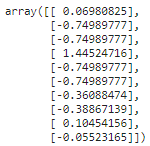
Let us perform standard scaling on the ‘tip’ column.

from sklearn.preprocessing import StandardScaler

## calculating mean and standard deviation of the column
scaler = StandardScaler().fit(np.array(X_train['tip']).reshape(-1,1))

## transforming the data using calculated mean and standard deviation
tips_transformed = scaler.transform(np.array(X_test['tip']).reshape(-1,1))

tips_transformed[:10]

The ‘reshape’ method is used to convert the 1D array into a 2D array since the fit and transform method requires a 2D array as input.

Scaling features to a range (MinMaxScaler and MaxAbsScaler)

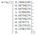
This is another approach to standardization in which features are scaled to lie between the minimum and maximum value, often between zero and one, or so that the maximum absolute value of each feature is scaled to unit size.

If we want to scale our data to lie between ‘min’ and ‘max’ values using MinMaxScaler, the following formula is used:

MinMaxScaler:

from sklearn.preprocessing import MinMaxScaler

## calculating mean and standard deviation of the column
mm_scaler = MinMaxScaler().fit(np.array(X_train['tip']).reshape(-1,1))

## transforming the data using calculated mean and standard deviation
tips_transformed = mm_scaler.transform(np.array(X_test['tip']).reshape(-1,1))

tips_transformed[:10]

MaxAbsScaler works in a similar way, but it scales the data such that each value lies in the range [-1, 1]. This is done by dividing each value by the maximum value in each of the features.

Centering the data destroys the inherent sparseness of the data and generally, it is not an appropriate thing to do. But in a case where the features are on different scales, it makes sense to scale sparse inputs. MaxAbsScaler was specifically designed for the purpose of scaling sparse data and it is a recommended way.

MaxAbsScaler:

from sklearn.preprocessing import MaxAbsScaler

## calculating mean and standard deviation of the column
ma_scaler = MaxAbsScaler().fit(np.array(X_train['tip']).reshape(-1,1))

## transforming the data using calculated mean and standard deviation
tips_transformed = ma_scaler.transform(np.array(X_test['tip']).reshape(-1,1))

tips_transformed[:10]

Scaling data with outliers (RobustScaler)

If the data is infested with outliers, then the value of the mean and standard deviation could get skewed. In this case, mean and std. deviation values won’t represent the data’s center or data’s spread correctly. Therefore, using mean and std. deviation for scaling when the data has outliers would not work well.

To circumvent this issue, we can use RobustScaler, which uses more robust estimates for the center and range of the data.

from sklearn.preprocessing import RobustScaler

## calculating mean and standard deviation of the column
r_scaler = RobustScaler().fit(np.array(X_train['tip']).reshape(-1,1))

## transforming the data using calculated mean and standard deviation
tips_transformed = r_scaler.transform(np.array(X_test['tip']).reshape(-1,1))

tips_transformed[:10]

Mapping to a Uniform Distribution (QuantileTransformer)

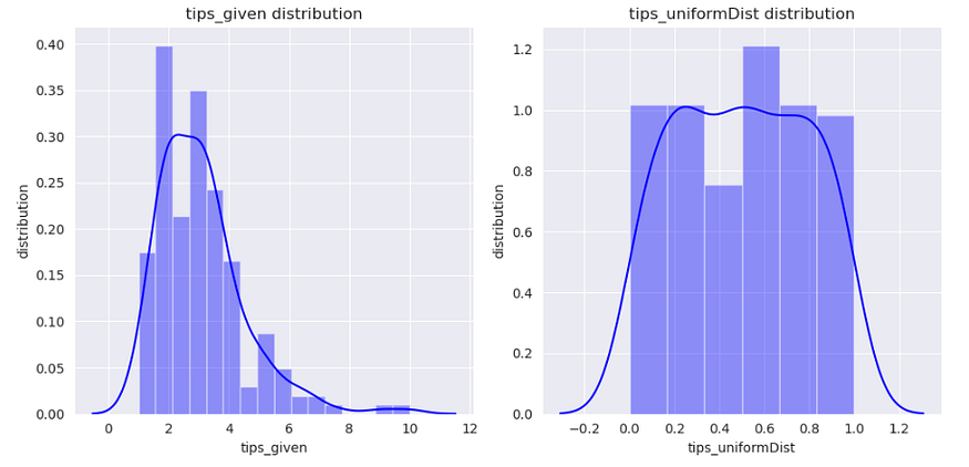
QuantileTransformer can be used to map the data to a uniform distribution with values between 0 and 1.

from sklearn.preprocessing import QuantileTransformer

q_transformer = QuantileTransformer().fit(np.array(X_train['tip']).reshape(-1,1))

xtrain_transformed = q_transformer.transform(np.array(X_train['tip']).reshape(-1,1))

Now, let’s visualize the ‘tip’ column before and after the transformation.

dataframe = pd.DataFrame()
dataframe['tips_given'] = X_train['tip']
dataframe['tips_uniformDist'] = xtrain_transformed

sns.set_style('darkgrid')
plt.figure(figsize=(10,5))
for index, feature in enumerate(dataframe.columns):
 plt.subplot(1,2,index+1)
 sns.distplot(dataframe[feature],kde=True, color='b')
 plt.xlabel(feature)
 plt.ylabel('distribution')
 plt.title(f"{feature} distribution")

plt.tight_layout()

Mapping to a Gaussian Distribution (PowerTransformer)

We can use the PowerTransformer to map the data to a distribution as close as to a Gaussian distribution.

We can choose from two methods that are used to make this transformation.

1. Box-cox transform
2. Yeo-Johnson transform

Note that the box-cox transformation can only be applied to the positive data.

box-cox transform:

from sklearn.preprocessing import PowerTransformer

p_transformer = PowerTransformer(method='box-cox').fit(np.array(X_train['tip']).reshape(-1,1))

xtrain_transformed = p_transformer.transform(np.array(X_train['tip']).reshape(-1,1))

dataframe = pd.DataFrame()
dataframe['tips_given'] = X_train['tip']
dataframe['tips_NormalDist'] = xtrain_transformed

sns.set_style('darkgrid')
plt.figure(figsize=(10,5))
for index, feature in enumerate(dataframe.columns):
 plt.subplot(1,2,index+1)
 sns.distplot(dataframe[feature],kde=True, color='y')
 plt.xlabel(feature)
 plt.ylabel('distribution')
 plt.title(f"{feature} distribution")

plt.tight_layout()

Yeo-Johnson transform:

from sklearn.preprocessing import PowerTransformer

p_transformer = PowerTransformer(method='yeo-johnson').fit(np.array(X_train['tip']).reshape(-1,1))

xtrain_transformed = p_transformer.transform(np.array(X_train['tip']).reshape(-1,1))

dataframe = pd.DataFrame()
dataframe['tips_given'] = X_train['tip']
dataframe['tips_NormalDist'] = xtrain_transformed

sns.set_style('darkgrid')
plt.figure(figsize=(10,5))
for index, feature in enumerate(dataframe.columns):
 plt.subplot(1,2,index+1)
 sns.distplot(dataframe[feature],kde=True, color='g')
 plt.xlabel(feature)
 plt.ylabel('distribution')
 plt.title(f"{feature} distribution")

plt.tight_layout()

I hope you like the article. If you have any thoughts on the article, then please let me know. Also, Keep an eye out for the upcoming article in this preprocessing series.

Connect with me at

LinkedIn

Website

Mail me at [email protected]

Have a great day!

Join thousands of data leaders on the AI newsletter. Join over 80,000 subscribers and keep up to date with the latest developments in AI. From research to projects and ideas. If you are building an AI startup, an AI-related product, or a service, we invite you to consider becoming a sponsor.

Published via Towards AI