Growing Teeth

Author(s): Dr. Marc Jacobs

Originally published on Towards AI.

Bayesian analysis of the Teeth Growth dataset.

To show that Bayesian analysis is really not that difficult, or far from how we humans deal with (new) information, I have posted several Bayesian analyses already. On known datasets, such as Iris, Chickweight, MTcars or Rent99. Today, I will show how I analyzed a simulated dataset called ABC. It is nothing fancy, but that does not have to be. Bayes’ Theorem works wonders, especially in small samples, and its power comes from beyond the current dataset. That is why using Bayesian analysis will always tell you more than any kind of Maximum Likelihood approach ever can. Remember, it is all about conditional probabilities.

In this post, I will apply what I already applied before, but then to the ToothGrowth dataset which shows the effect of vitamin C on tooth growth in guinea pigs. It is a dataset that has been used in many many posts on various media before, and I am sure there is a Bayesian analysis somewhere, but I will try and go ahead anyhow. Please read this post in conjunction with the others I made. I believe you will find them quite coherent and therefore helpful in terms of learning how to apply the Bayes Theorem. Let me know if otherwise!

BTW, I placed the codes at the end, so I can tell the story better. Not everything I did is IN the post but is in the codes. Enjoy!

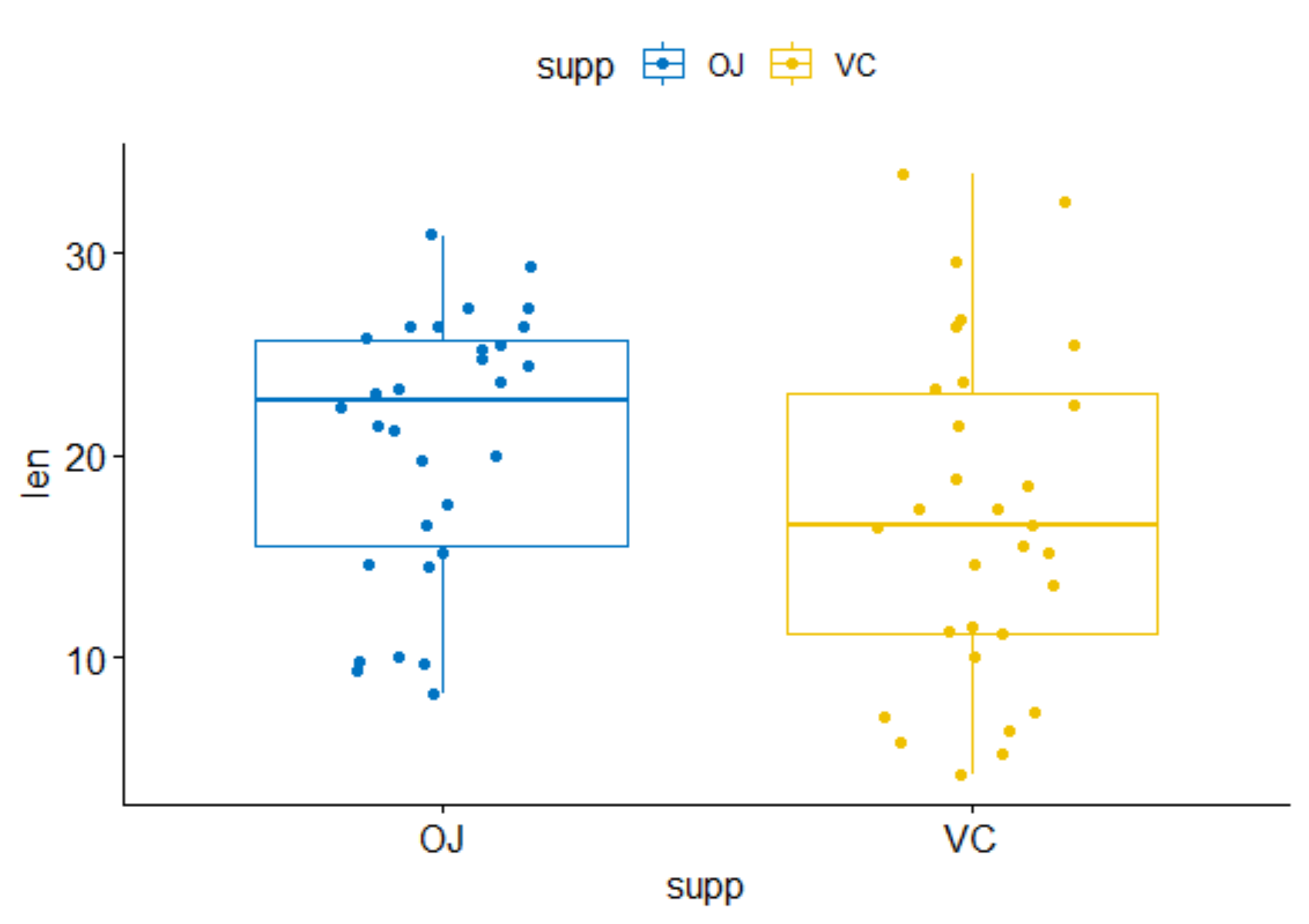
So, what are we dealing with? Well, as you can see below, we have the length of the teeth, the supplement applied (OJ vs VC), and the dose. It really is not more than this, and the dataset is quite small.

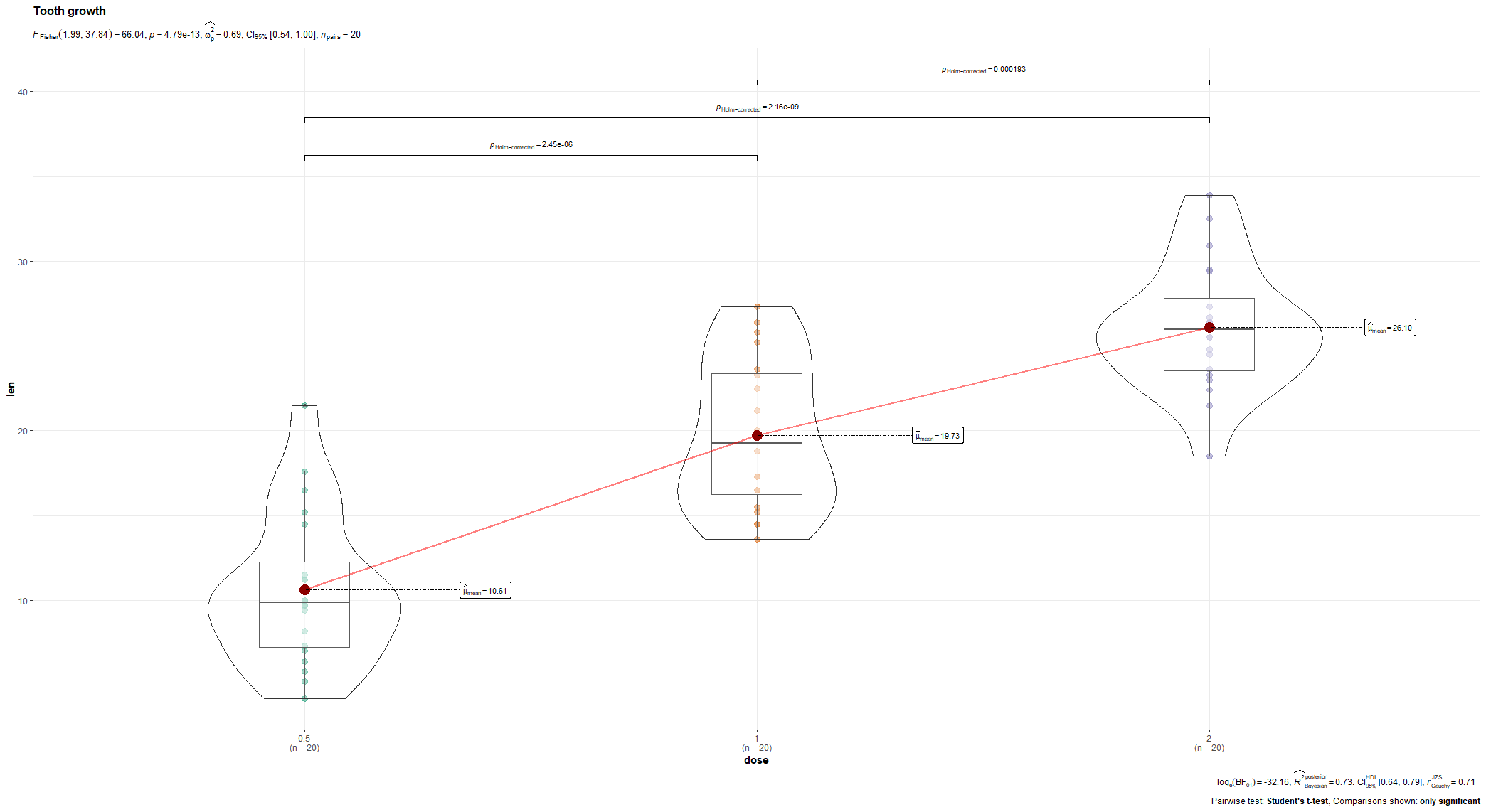
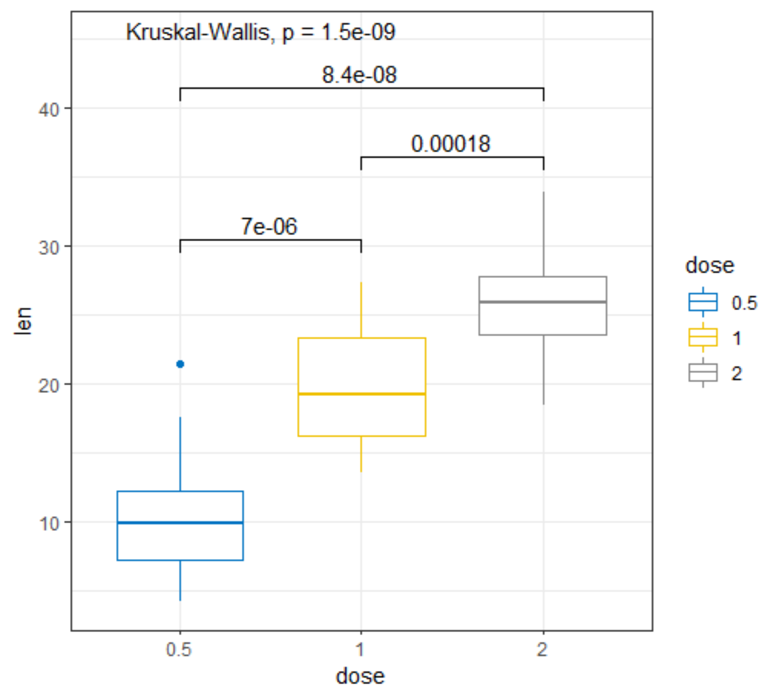
R has many many functions that can make the most basic of data look like rocket science. Just to show you how ridiculous some of these plots are, and how much number-porn you can add to a straightforward graph, here are some examples. These numbers are not helpful in the least and will make you believe there is much more to extract from such a small sample than actually is the case.

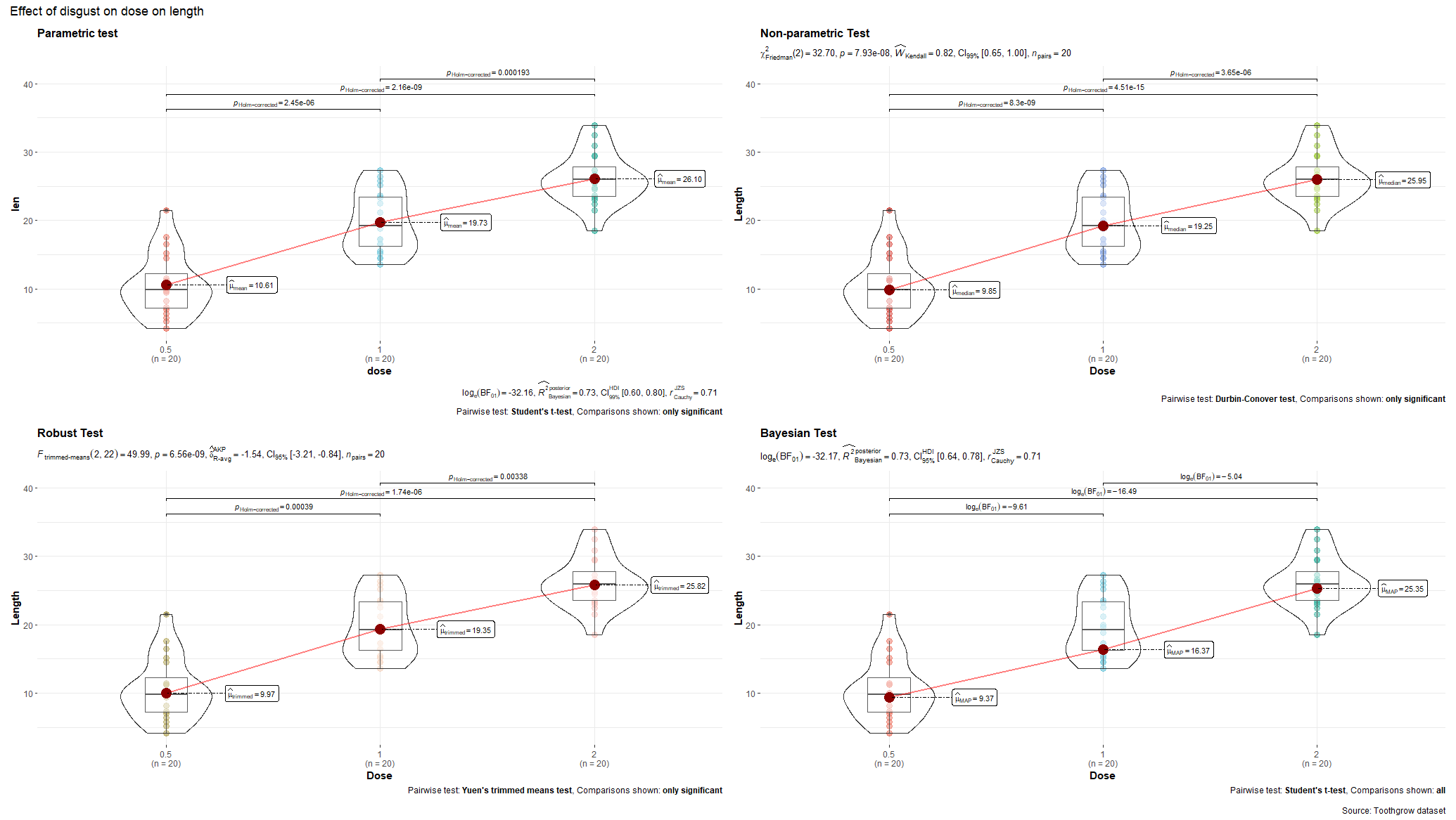
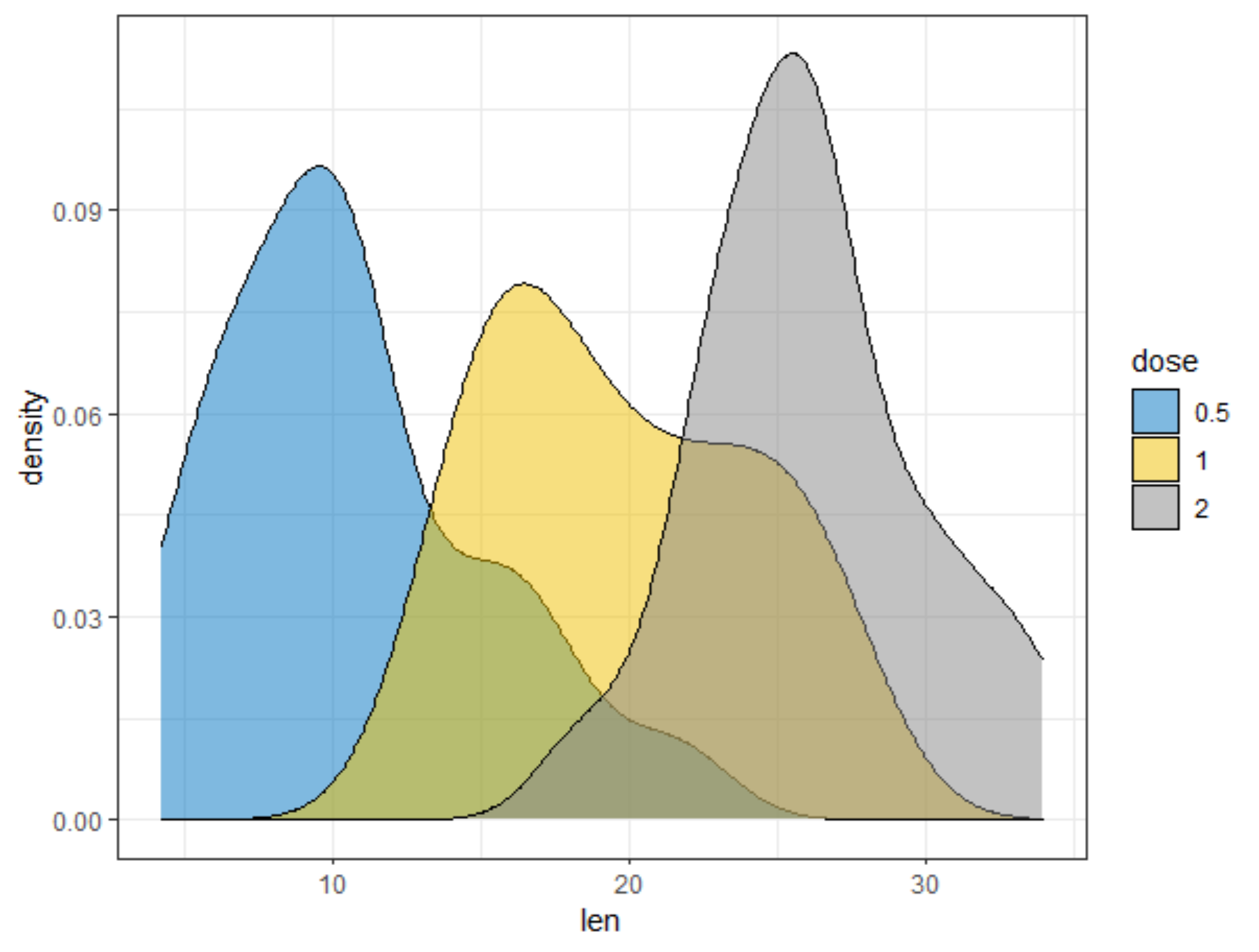
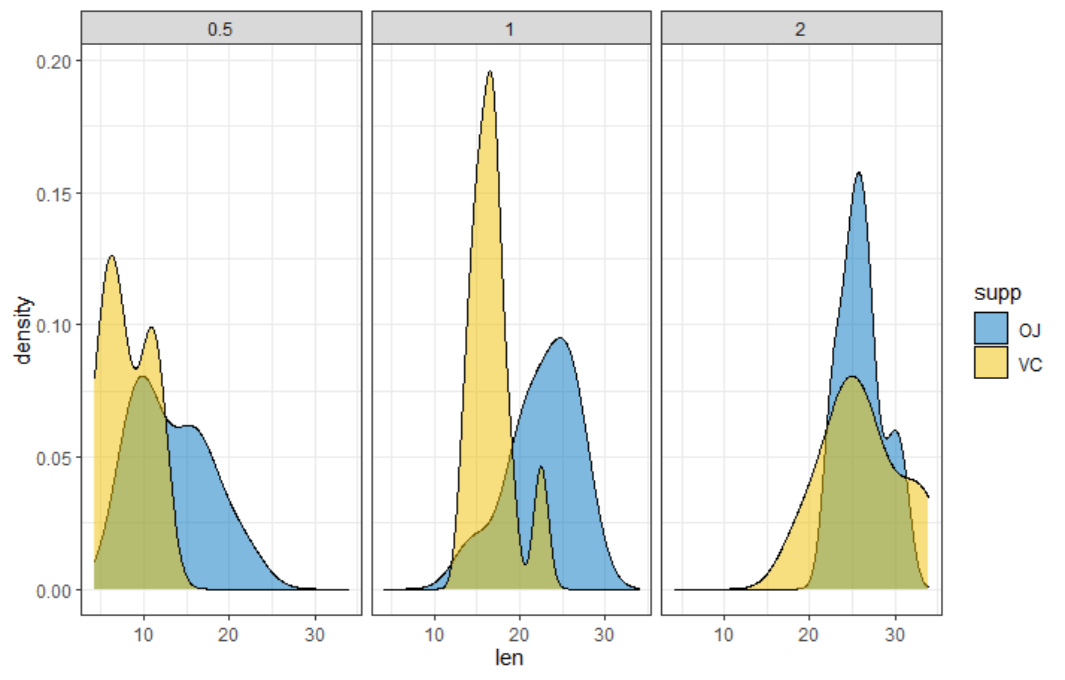
Below, I have made six plots, showing to the left a box-plot with a value and to the right a density plot showing just that, densities. P-values are dependent on p-values as well of course, but I want you to get acquainted with the right plots, not the left. Boxplots are one of the greatest plots to make, but in Bayesian analysis, it is all about density plots.

Let's move on to the actual modeling part. The dataset is small and not exciting so this is more of a technical post, showcasing the functions available in R for Bayesian analysis. Below, I am using rstanarm, although my personal favorite is brms. Both use STAN for sampling and communicate with STAN via a compiler.

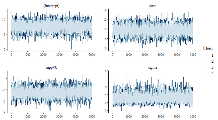
Now, let's do some additional analysis, checking how the sampling when and comparing the likelihood to the posterior. I cannot stress how important it is to note that the likelihood and the posterior MAY deviate. Nothing wrong, no problem.

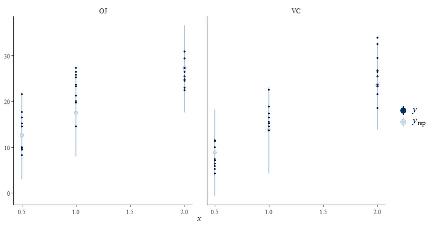
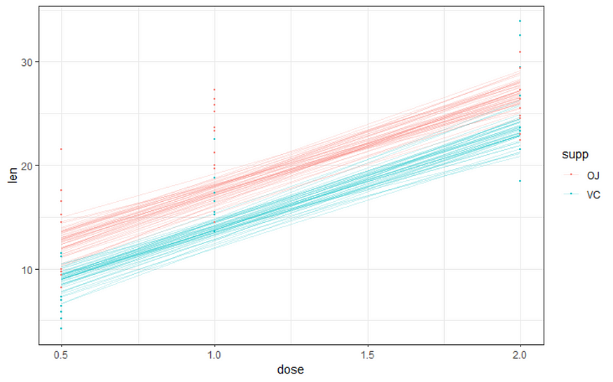
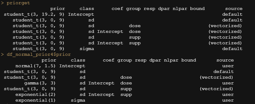
In the previous example, I modeled dose as a numeric variable. You can of course also have a go at that variable as a factor. For this example, I used brms. What you can see is the prior that comes from the model if I specify nothing and the prior I used. My priors state that there are no differences between dose 1 and dose 2 compared to dose 0. Also, there is no difference between the supplements. Hence, my prior knowledge makes that I expect nothing, and I want to see how that coincides with the latest dataset.

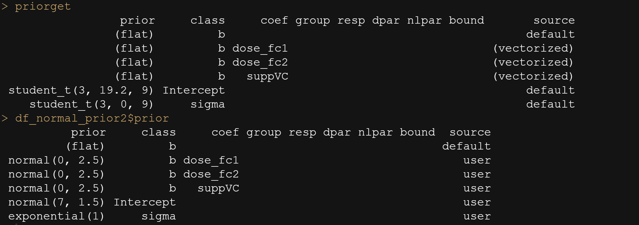
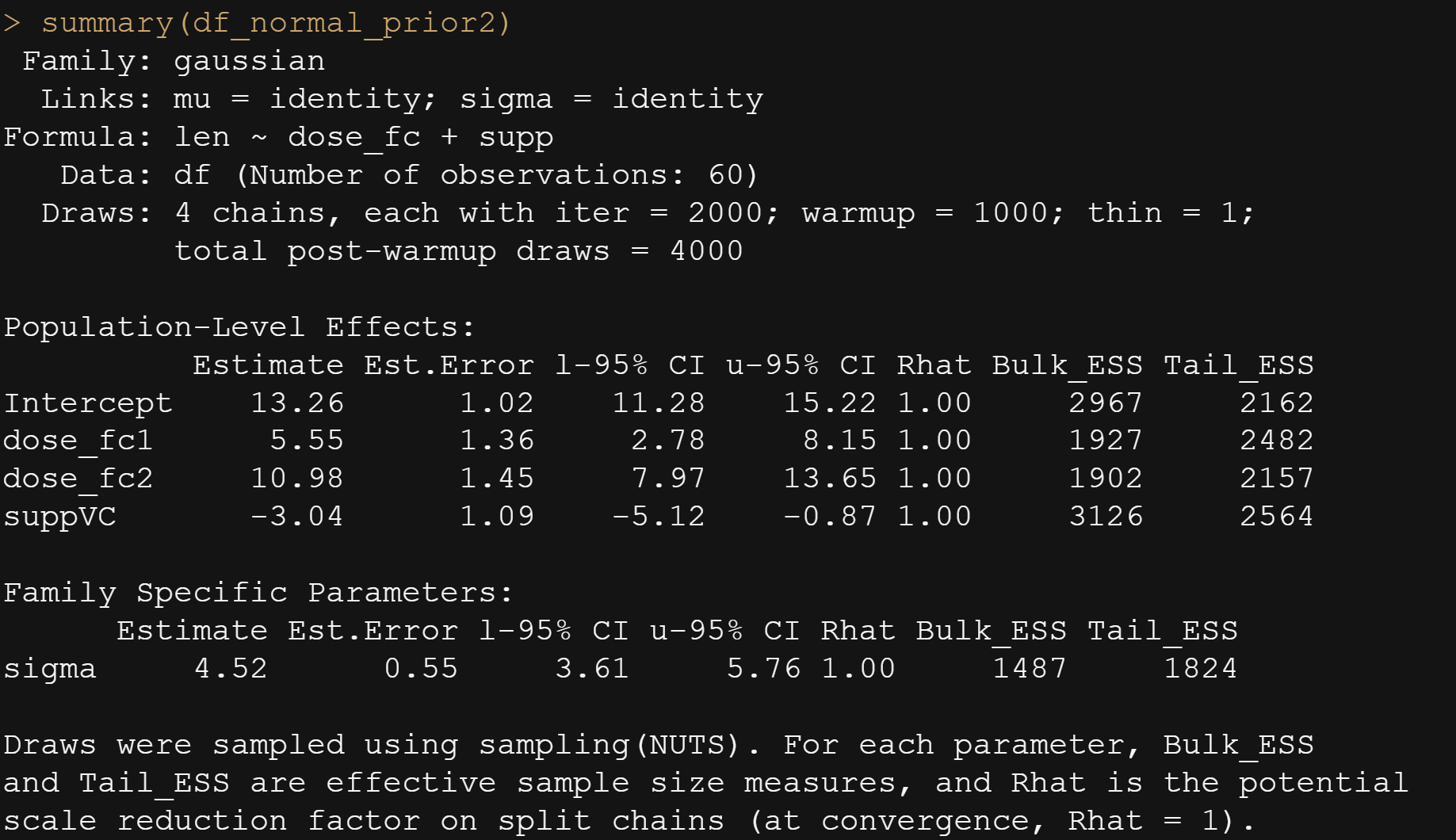
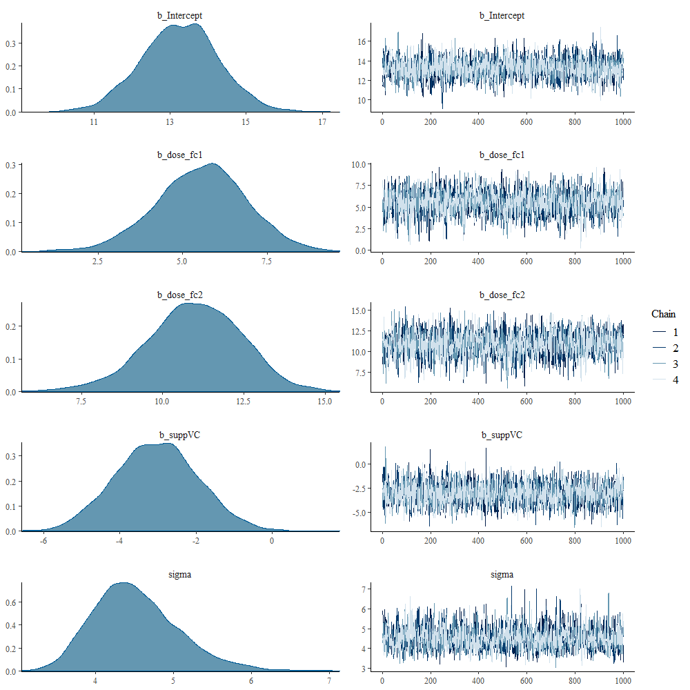
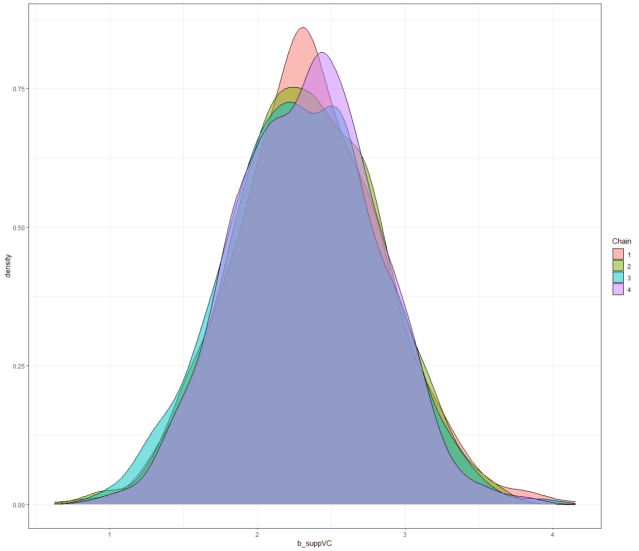
And, another model in which I changed analyzed dose as a numeric variable, and changed the priors. This is all child’s play, but finding the prior is not. Since I know nothing about Guinea pigs my prior can be informative, statistically speaking, but does not have a solid base by itself.

And another model, in which we place all parameters in the random part of the model. As a result, we have a Bayesian Mixed Model, which is a bit paradoxical. If you know why you figured Bayesian analysis out! (hint: in Bayesian analysis, all parameters are considered random and variable).

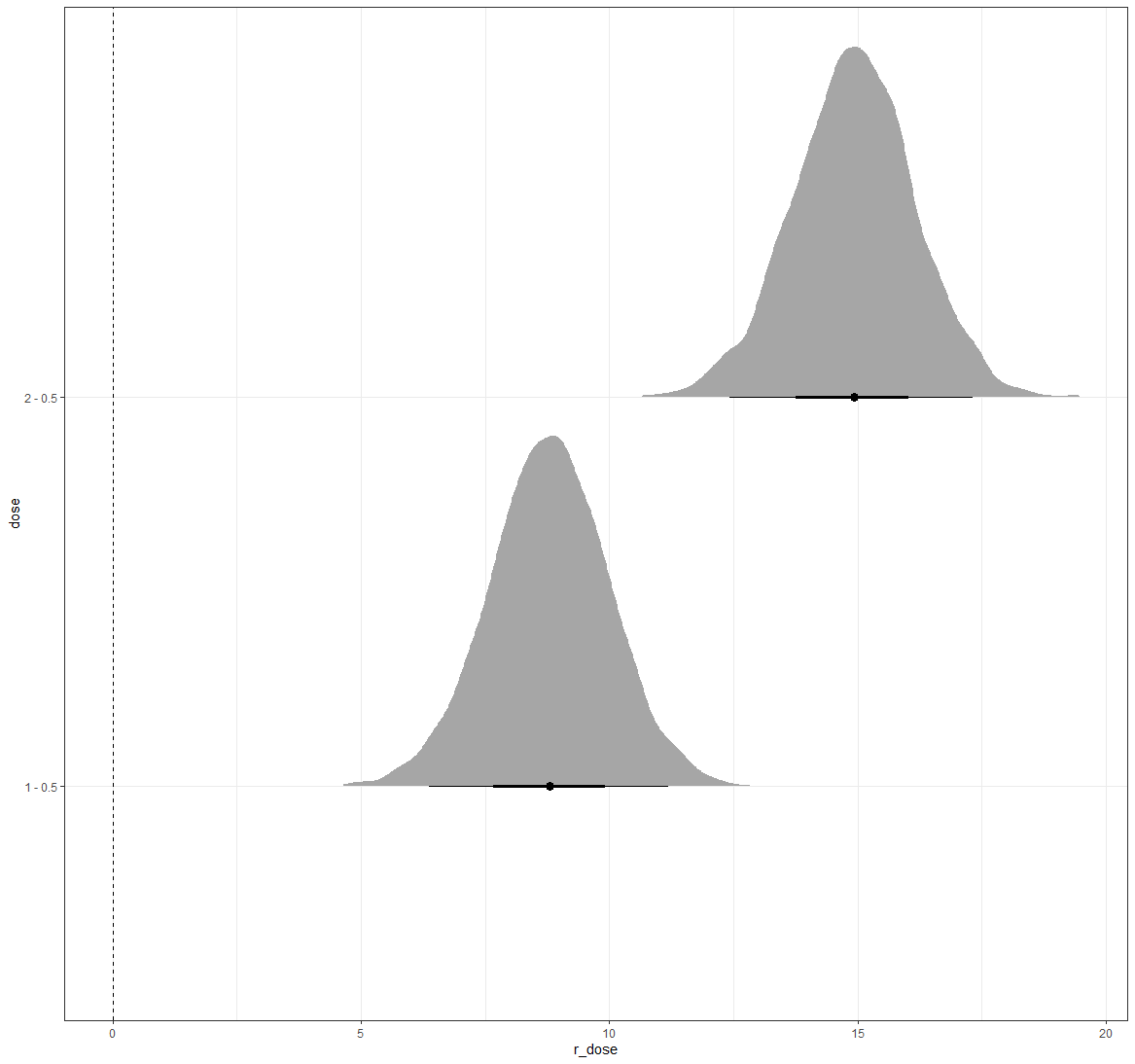
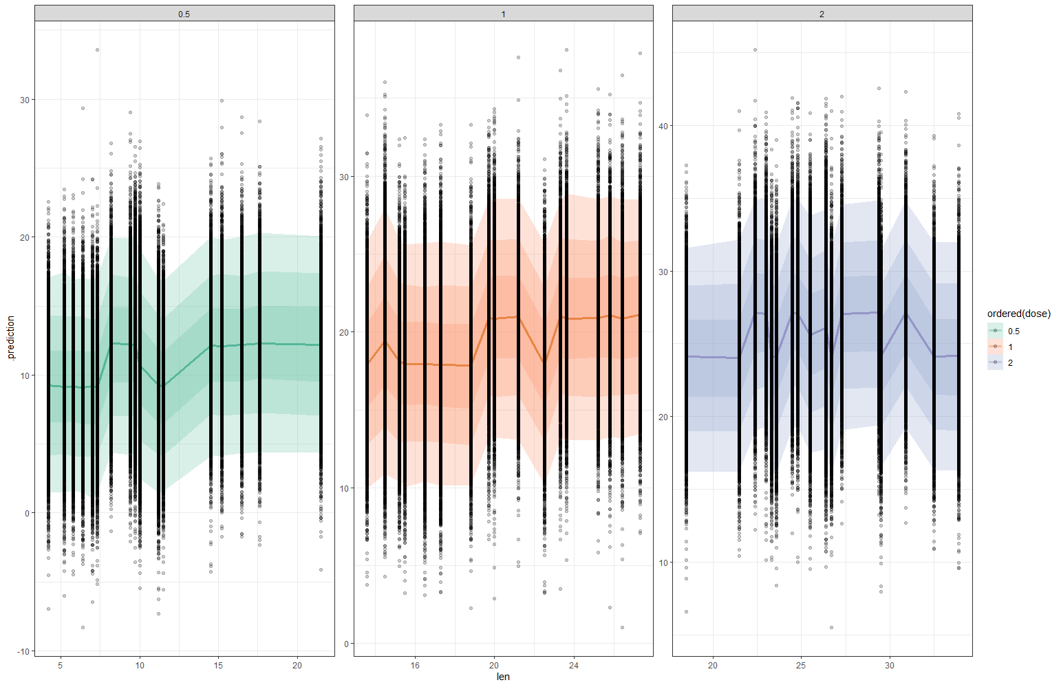
And, last but not least, predictions come from the Bayesian model. Both the ribbon and the points show the posterior distributions. These plots show you how fickle modeling is in general — just look at the parts in the dose variable for which no data is available. Interpolation rules and that is always a weakness.

I hope you enjoyed this post! Let me know if something is amiss!

Join thousands of data leaders on the AI newsletter. Join over 80,000 subscribers and keep up to date with the latest developments in AI. From research to projects and ideas. If you are building an AI startup, an AI-related product, or a service, we invite you to consider becoming a sponsor.

Published via Towards AI