Thresholding and Otsu’s Method
Last Updated on July 25, 2023 by Editorial Team
Author(s): Erika Lacson
Originally published on Towards AI.
Introduction to Image Processing with Python
Episode 5: Image Segmentation — Part 1
Welcome back, my fellow image-processing enthusiasts! In our fifth episode, we’re diving straight into the heart of image analysis — Image Segmentation! This is the process of partitioning an image into multiple segments, each corresponding to different objects or parts of objects. U+1F9E9 It’s the backbone of many computer vision tasks like object detection, facial recognition, and medical imaging.
In this two-part exploration of Image Segmentation, here’s the exciting stuff we’re going to unpack:
- Thresholding and Otsu’s Method U+2696️ (This episode)
- Color Image Segmentation U+1F308 (This episode)
- Chromaticity Segmentation U+1F3A8 (Next episode)
- Image Differencing U+1F504 (Next episode)
For this episode, our journey will begin with:
Our first stop is the world of Thresholding and Otsu’s Method. It’s the first step into our segmentation adventure, where we’ll find out how simple yet effective methods like these can partition an image into two parts — foreground and background, based on the intensity values of its pixels.
But how do we decide the threshold value? That’s where Otsu’s method comes in handy. Remember Otsu? The one we used to automatically assign the threshold for our Binary Image? This is it now. In this episode, Otsu’s Method or Otsu’s Thresholding, will be our main topic. To recap, this nifty method or thresholding technique calculates the optimal threshold value that maximizes the between-class variance, making it an excellent tool for automatic threshold selection. U+1F3C6
Let’s start by importing our libraries and displaying our image:
# Import libraries
from skimage.io import imread, imshow
import matplotlib.pyplot as plt
import numpy as np
from skimage.color import rgb2gray, rgb2hsv
from skimage.filters import threshold_otsu
# Display the image that we will be playing with
original_image = imread('plants.jpg')
plt.figure(figsize=(20,20))
plt.imshow(original_image)
plt.title('Original Image', fontsize=20, weight='bold')
plt.axis('off')
plt.show()

Previously, when we want to binarize our image, we performed a two-step process of converting the image to grayscale and then setting any threshold we want, usually 0.50, to convert it to a binary image:
# Convert the image to grayscale
gray_image = rgb2gray(original_image)
plt.figure(figsize=(20,20))
plt.imshow(gray_image, cmap='gray')
plt.title('Grayscale Image', fontsize=20, weight='bold')
plt.axis('off')
plt.show()

# Convert the grayscale image to binary image using threshold=0.50
threshold = 0.5
binary_image = gray_image<threshold
plt.figure(figsize=(20,20))
plt.imshow(binary_image, cmap='gray')
plt.title('Binary Image', fontsize=20, weight='bold')
plt.axis('off')
plt.show()
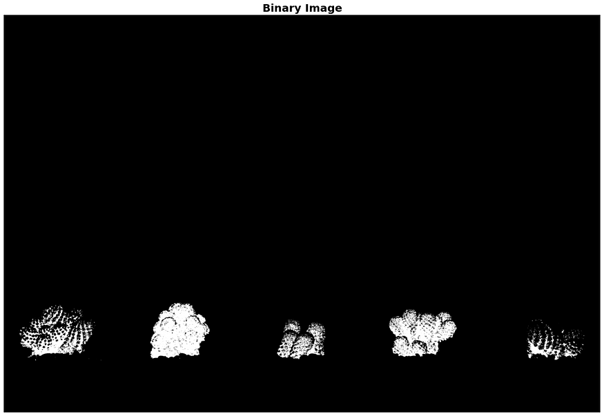
Notice how the originally lighter parts of the image turned black. This is because we used 0.50 as our threshold.
But in Otsu’s Method, we don’t have to manually set the threshold, we can let Otsu handle that job for us by calling threshold_otsu function and use it in our gray_image as follows:
# Use threshold_otsu to automatically calculate the optimal threshold
threshold = threshold_otsu(gray_image)
print(f"Otsu's Threshold: {threshold:.2f}")
binary_image_otsu = gray_image < threshold
plt.figure(figsize=(20,20))
plt.imshow(binary_image_otsu, cmap='gray')
plt.title("Binary Image using Otsu's Method", fontsize=20, weight='bold')
plt.axis('off')
plt.show()
Output:
Otsu's Threshold: 0.67
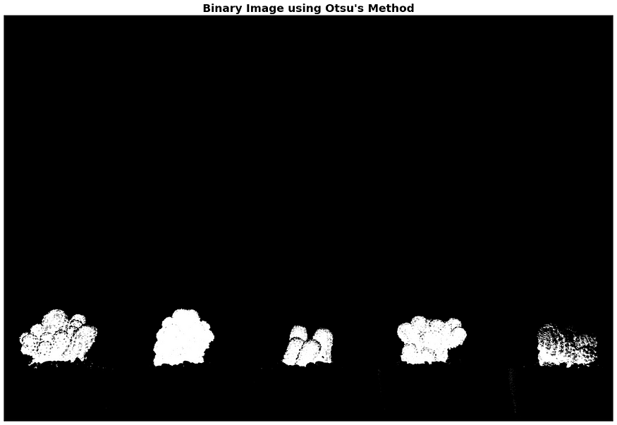
See the difference? We don’t have to manually trial and error on our threshold values just to get a better-binarized image. We saved time, thanks to Otsu’s Method!
Color Image Segmentation U+1F308
Suppose we want to isolate only the verdant plant life in our image, then it’s time for another exciting technique — Color Image Segmentation! This method is an extension of thresholding, but here’s the twist: instead of intensity, we’re using color information to separate objects. It’s particularly useful when the objects of interest in an image are dressed in distinctive colors. U+1F3AF
Now, let’s venture into the different color spaces, like RGB and HSV, and witness how switching between these spaces can drastically uplift our segmentation results.
RGB Color Space U+1F534U+1F7E2U+1F535
Let’s cast our eyes on our original image once more.
# Display original image
original_image = imread('plants.jpg')
plt.figure(figsize=(20,20))
imshow(original_image)
plt.title('Original Image', fontsize=20, weight='bold')
plt.axis('off')
plt.show()

To isolate only the lush green plant, we can perform a simple segmentation operation. The RGB channels can be accessed in the image like so:
img = original_image.copy()

# Separate the red, green, and blue channels
r = img[:,:,0]
g = img[:,:,1]
b = img[:,:,2]
We can use the comparative operators below to say that a pixel is green if the green channel value is greater than both the red and blue channel values. This can work well if green is the dominant color in the image. And as you can see below, I was able to successfully segment the green color in the image by just using comparative operators about what we know about the RGB channels.
# Read image using skimage
original_image = imread('plants.jpg')

# Create subplot of 1x2
fig, ax = plt.subplots(1, 2, figsize=(20, 20))

# Plot original image
ax[0].imshow(original_image)
ax[0].set_title('Original Image', fontsize=20, weight='bold')
ax[0].axis('off')

# Get red, green, and blue channels
r = original_image[:, :, 0]
g = original_image[:, :, 1]
b = original_image[:, :, 2]

# Create a mask for green color
mask = (g > r) & (g > b) # adjust these values depending on what you consider to be 'green'

# Create a new image
new_img = original_image.copy()

# Apply mask to all channels
new_img[:, :, 0] = new_img[:, :, 0] * mask
new_img[:, :, 1] = new_img[:, :, 1] * mask
new_img[:, :, 2] = new_img[:, :, 2] * mask

# Plot the green segmented image
ax[1].imshow(new_img)
ax[1].set_title('Green Segmented Image', fontsize=20, weight='bold')
ax[1].axis('off')

# Display the subplot
plt.tight_layout()
plt.show()
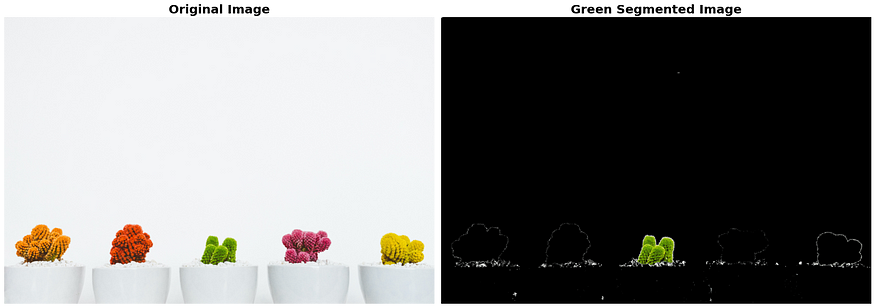
Notice how there are white marks left in the green segmented image?
White is a color where red, green, and blue all are at their peak. Therefore, to keep these unwanted guests at bay, we can add a white mask to our code:
# Create a mask for white color
white_threshold = 180 # adjust this depending on what you consider to be 'white'
white_mask = (r > white_threshold) & (g > white_threshold) & (b > white_threshold)
# Combine the green and white masks
mask = green_mask & ~white_mask # ~ is the NOT operator
# Read image using skimage
original_image = io.imread('plants.jpg')

# Create subplot of 1x2
fig, ax = plt.subplots(1, 2, figsize=(20, 20))

# Plot original image
ax[0].imshow(original_image)
ax[0].set_title('Original Image', fontsize=20, weight='bold')
ax[0].axis('off')

# Get red, green, and blue channels
r = original_image[:,:,0]
g = original_image[:,:,1]
b = original_image[:,:,2]

# Create a mask for green color
green_mask = (g > r) & (g > b)

# Create a mask for white color
white_threshold = 180 # adjust this depending on what you consider to be 'white'
white_mask = (r > white_threshold) & (g > white_threshold) & (b > white_threshold)

# Combine the green and white masks
mask = green_mask & ~white_mask # ~ is the NOT operator

# Create a new image and apply mask
new_img = original_image.copy()

# Apply mask to all channels
new_img[:,:,0] = new_img[:,:,0] * mask
new_img[:,:,1] = new_img[:,:,1] * mask
new_img[:,:,2] = new_img[:,:,2] * mask

# Plot the green segmented image
ax[1].imshow(new_img)
ax[1].set_title('Green Segmented Image', fontsize=20, weight='bold')
ax[1].axis('off');

Well done!
Apart from comparative operators, we have a few other tools in our arsenal:
- Using thresholds: You can select a threshold and say that a pixel is green if its green channel value is above this threshold. This threshold can be chosen based on the specific shades of green you’re interested in.
mask = (g > some_green_threshold)
- Using ranges: Instead of just saying a pixel is green if its green channel value is above a certain threshold, you can define a range for the green channel values and also specify that the red and blue channel values should be below certain thresholds.
mask = ((g > lower_green_threshold) & (g < upper_green_threshold)) & (r < some_red_threshold) & (b < some_blue_threshold)
- Using color spaces: Instead of working in the RGB color space, sometimes it’s easier to segment colors in other color spaces like
HSV(Hue, Saturation, Value). In the HSV color space, different colors are arranged on a circle (the hue), and so picking out a specific color may be easier.
The above RGB technique worked as a treat, but what if we had to isolate the orange plant? The RGB space would leave us in a bit of a pickle. That's where the magic of HSV color space can save the day!
HSV Color Space
As mentioned above, instead of working in the RGB color space, sometimes it’s easier to segment colors in other color spaces like HSV (Hue, Saturation, Value). In the HSV color space, different colors are arranged on a circle (the hue), and so picking out a specific color may be easier.
Let’s display the Hue, Saturation, and Value of our original image:
# Read image using skimage
original_image = imread('plants.jpg')

# Convert the image to HSV color space
hsv_img = rgb2hsv(original_image)

fig, ax = plt.subplots(1, 3, figsize=(20,20))
ax[0].imshow(hsv_img[:,:,0], cmap='hsv')
ax[0].set_title('Hue', fontsize=20)
ax[1].imshow(hsv_img[:,:,1], cmap='hsv')
ax[1].set_title('Saturation', fontsize=20)
ax[2].imshow(hsv_img[:,:,2], cmap='hsv')
ax[2].set_title('Value', fontsize=20);

Since it’s difficult to see the difference in intensity values using the above plot, let’s use colorbar():
plt.imshow(hsv_img[:,:,0], cmap='hsv')
plt.colorbar()
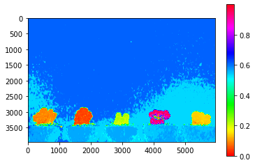
As you can see, orange is between 0 to 0.05, so let’s use those as our threshold:
# Read image using skimage
original_image = imread('plants.jpg')

# Convert the image to HSV color space
hsv_img = rgb2hsv(original_image)

# Create a mask for orange color
# Hue for orange is roughly in the range of 0 - 0.05
# We can play around these values to adapt to our specific color requirement
mask = (hsv_img[:,:,0] > 0) & (hsv_img[:,:,0] < 0.05)

# create a new image and apply mask
new_img = original_image.copy()

new_img[:,:,0] = new_img[:,:,0] * mask
new_img[:,:,1] = new_img[:,:,1] * mask
new_img[:,:,2] = new_img[:,:,2] * mask

# plot the original and segmented images side by side
fig, ax = plt.subplots(1, 2, figsize=(20,10))

ax[0].imshow(original_image)
ax[0].set_title('Original Image', fontsize=20, weight='bold')
ax[0].axis('off')

ax[1].imshow(new_img)
ax[1].set_title('Orange Segmented Image', fontsize=20, weight='bold')
ax[1].axis('off')

plt.show()

And voilà! We’ve successfully segmented out the vibrant hues of orange in our plant image.
Conclusion U+1F3C1
Whew, what a journey we’ve had today! Our deep dive into image segmentation has certainly painted a vibrant picture of how we can distill meaningful information from our images. U+1F5BC️U+1F50D From the fundamental idea of thresholding, through the magic of Otsu’s method, to our vivid journey through color image segmentation, we’ve touched upon some key techniques that form the cornerstone of image processing. U+1F308U+2696️
Remember, these aren’t just methods, they’re powerful tools you can harness to illuminate the hidden secrets within your images! Whether it’s isolating the verdant leaves of a plant in the RGB color space, or teasing out the vibrant hues of a flower using Otsu’s method, you’re now equipped with the knowledge to take on more complex image processing challenges! U+1F343U+1F33C
But don’t close your notebooks just yet! We’ve only scratched the surface of image segmentation. In the next episode, we’ll be delving into the colorful world of chromaticity segmentation and exploring the fascinating concept of image differencing. So, stay curious and keep those coding fingers ready! U+1F3A8U+1F4BB
So, until next time, keep exploring, keep learning, and remember: every pixel tells a story! U+1F9E0U+1F4A1U+1F388
Happy coding, and see you in the next episode! U+1F680U+1F469U+1F4BBU+1F468U+1F4BBU+1F31F
References:
- Borja, B. (2023). Lecture 5: Image Segmentation Part 1 [Jupyter Notebook]. Introduction to Image Processing 2023, Asian Institute of Management.
Join thousands of data leaders on the AI newsletter. Join over 80,000 subscribers and keep up to date with the latest developments in AI. From research to projects and ideas. If you are building an AI startup, an AI-related product, or a service, we invite you to consider becoming a sponsor.
Published via Towards AI
Towards AI Academy
We Build Enterprise-Grade AI. We'll Teach You to Master It Too.
15 engineers. 100,000+ students. Towards AI Academy teaches what actually survives production.
Start free — no commitment:
→ 6-Day Agentic AI Engineering Email Guide — one practical lesson per day
→ Agents Architecture Cheatsheet — 3 years of architecture decisions in 6 pages
Our courses:
→ AI Engineering Certification — 90+ lessons from project selection to deployed product. The most comprehensive practical LLM course out there.
→ Agent Engineering Course — Hands on with production agent architectures, memory, routing, and eval frameworks — built from real enterprise engagements.
→ AI for Work — Understand, evaluate, and apply AI for complex work tasks.
Note: Article content contains the views of the contributing authors and not Towards AI.


