Data Science Essentials — Multicollinearity

Author(s): Nitin Chauhan

Originally published on Towards AI the World’s Leading AI and Technology News and Media Company. If you are building an AI-related product or service, we invite you to consider becoming an AI sponsor. At Towards AI, we help scale AI and technology startups. Let us help you unleash your technology to the masses.

Data Science Essentials — Multicollinearity

Introduction

I am aware of Multicollinearity because of my background in statistics, but I have observed that many professionals are unaware that it exists.

It is widespread for machine learning practitioners who do not come from a mathematical background. Even though Multicollinearity may not seem like the most critical topic to grasp in your journey, it is nonetheless a vital topic worth learning. Particularly if you are applying for a data scientist position.

In this article, we will examine what Multicollinearity is, why it is a problem, what causes Multicollinearity, as well as how to detect and correct it.

Topics Covered

• What is Multicollinearity?
• Types of Multicollinearity
• Understanding Multicollinearity
• Causes of Multicollinearity
• Detecting Multicollinearity
• Dealing with Multicollinearity

What is Multicollinearity?

Multicollinearity can be defined as the presence of high correlations between two or more independent variables (predictors). This is essentially a phenomenon in which independent variables are correlated with one another.

It measures the degree to which two variables are related based on their correlation. The correlation between two variables can be positive (changes in one variable lead to changes in another variable in the same direction), negative (changes in one variable charge to changes in the opposite direction), or not.

Keeping some examples in mind helps us remember these terms.

1. Weight and height can be an example of a positive correlation. The taller you are, the heavier you weigh (if we ignore the exception case, this is considered a general trend).
2. For example, the higher you go, the lower your oxygen level. This is a simple example of a negative correlation.

Returning to our multicollinearity concept, when more than one predictor in a regression analysis is highly correlated, they are termed multicollinear. A higher education level is generally associated with a higher income, so one variable can easily be predicted using another variable. As a result of keeping both of these variables in our analysis, we may encounter problems.

Types of Multicollinearity

There are two basic kinds of multicollinearity:

1. Structural multicollinearity: This results from researchers (people like us) creating new predictors based on the given predictors to solve the problem. For instance, variable x2 is created from the predictor variable x; thus, this type of multicollinearity results from the model specified and is not a consequence of the data itself.
2. Data Multicollinearity: This type of multicollinearity arises from poorly designed experiments that are observational. It is not something that has been specified or developed by the researcher.

Comments: In an observational study, we surveyed members of a sample without attempting to influence them. For example, observational research asks people whether they drink milk or coffee before going to bed and reports that the data shows that people who drink milk are more likely to sleep earlier. You can learn more about this by clicking here.

Visual inspection of multicollinearity:

• Perfect multicollinearity: In a regression model, perfect multicollinearity occurs when two or more independent predictors exhibit a linear relationship that is perfectly predictable (exact or not random). For example, weight in pounds and kilograms has a coefficient of +1 or -1. However, we rarely encounter problems with perfect multicollinearity.
• High multicollinearity: Usually this is often a common issue in the data preparation phase. Generally, high multicollinearity can be either positive or negative. For example, inflation is where demand and supply are highly correlated but in the opposite direction.

Our analyses are based on detecting and managing high/imperfect/near multicollinearity, which occurs when more than one independent predictor is linearly related.

Understanding Multicollinearity

A multicollinear regression model can be problematic because it is impossible to distinguish between the effects of the independent variables on the dependent variable. For example, consider the following linear equation:

Y = W0+W1*X1+W2*X2

The coefficient W1 represents the increase in Y for a unit increase in X1 while X2 remains constant. However, since X1 and X2 are highly correlated, changes in X1 would also affect X2, and we would not be able to distinguish their effects on Y independently.

As a result, it isn’t easy to distinguish between the effects of X1 and X2 on Y.

We may not lose accuracy due to Multicollinearity. Still, we may lose reliability when determining the effects of individual features in your model, which can be an issue in interpreting it.

Causes of Multicollinearity

The following problems may contribute to Multicollinearity:

• Data multicollinearity may result from problems with the dataset at the time of its creation, which could include poorly designed experiments, highly observational data, or an inability to manipulate the data:
• For example, we are determining a household’s electricity consumption from the household income and the number of electrical appliances. In this instance, we know that the number of electrical appliances will increase with household income. As a consequence, this cannot be removed from the dataset.
• In addition, Multicollinearity may occur when new variables are created that are dependent on other variables:
• Adding a variable for BMI to the height and weight variables would add redundant information to the model.
• The dataset should include the following identical variables:
• It would be helpful to include variables for temperature in Fahrenheit and temperature in Celsius, for example.
• An error in using dummy variables can also lead to a multicollinearity problem known as the Dummy variable trap.
• It would be redundant to create dummy variables for marriage status variables containing the same values: ‘married’ and ‘single.’ Instead, we can use one variable containing 0/1 for each status.
• Insufficient data in some cases can also cause multicollinearity problems.

Impact of Multicollinearity

Correlated predictors do not improve our regression analysis for the data. Correlated predictors may make our interpretation of the data less accurate.

In this problem, four predictors are present — age, gender, number of study hours, and level of parental education. The dependent variable (a variable that must be predicted) is the student’s performance on the test.

Consider the case in which the number of study hours and level of parental education are highly correlated.

A regression model determines which variable determines the student’s exam performance. It is assumed that the number of study hours and parental education are positively correlated with performance (perhaps one more strongly than the other). However, the model indicated that neither of these two variables was significant.

Students’ performance appears unaffected by the number of hours they study or their parent’s education level.

Understanding why the model made this statement is essential.

A regression model incorporating highly correlated predictors will estimate each of their effects while controlling the impact of a predictor, explaining all of the variation in performance that the predictor would have been able to clarify on its own. The same problem was experienced by our predictors, resulting in neither being a significant predictor.

The R-squared value returned by the model may indicate that one or more predictors are likely to be accurate.

Therefore, multicollinearity caused the model to produce misleading and confusing results.

Detecting Multicollinearity

Let’s try detecting multicollinearity in a dataset to give you a flavor of what can go wrong. Try out yourself the Ether Fraud Detection, link to Kaggle notebook here

# Import library for VIF
from statsmodels.stats.outliers_influence import variance_inflation_factor

def calc_vif(X):

    # Calculating VIF
    vif = pd.DataFrame()
    vif["variables"] = X.columns
    vif["VIF"] = [variance_inflation_factor(X.values, i) for i in range(X.shape[1])]

    return(vif)
result = calc_vif(newdf)

# Identify variables with high multi-collinearity
result[result['VIF']>10]

Multicollinearity can be detected via various methods. In this article, we will focus on the most common one — VIF (Variable Inflation Factors).

VIF determines the strength of the correlation between the independent variables. It is predicted by taking a variable and regressing it against every other variable.

R² value is determined to find out how well an independent variable is described by the other independent variables. A high value of R² means that the variable is highly correlated with the other variables. This is captured by the VIF, which is denoted below:

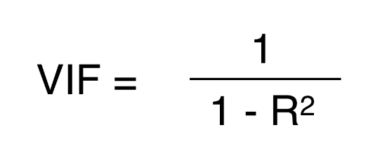
So, the closer the R² value to 1, the higher the value of VIF and the higher the multicollinearity with the particular independent variable.

We can see here that the ‘total Ether Sent’ and ‘total Ether Received’ have a high VIF value equal to infinite, meaning they can be predicted by other independent variables in the dataset.

Although correlation matrix and scatter plots can also be used to find multicollinearity, their findings only show the bivariate relationship between the independent variables. VIF is preferred as it can show the correlation of a variable with a group of other variables.

Dealing with Multicollinearity

Dropping one of the correlated features will help in bringing down the multicollinearity between correlated features:

Consider a strong multicollinearity case between ‘Weight’ & ‘Height’ in predicting the physical fitness of a person. If we were able to drop the variable ‘Weight’ & ‘Height’ from the dataset because their information was being captured by the ‘BMI’ variable. This has reduced the redundancy in our dataset.

Dropping variables should be an iterative process starting with the variable having the largest VIF value because its trend is highly captured by other variables. If you do this, you will notice that VIF values for other variables would have reduced too, although to a varying extent.

In our example, after dropping the ‘Weight’ & ‘Height’ variables, VIF values for all the variables have decreased to a varying extent.

df_temp = df.copy()

# Create a new feature that incorporates both features information
df_temp[‘BMI’] = df.apply(lambda x: x['Weight']/(x['Height']*x['Height']))

# Drop the columns used for the new feature with high multicollinearity
df_temp.drop(['Weight', 'Height'], inplace=True, axis=1)

Key Takeaways

Multicollinearity can often lead to predictions being overfitted on a certain set of features which impacts the significance of another variable that may have better-predicting power. Generally, it’s quite easy to deal with multicollinearity either through selecting a relevant feature (domain knowledge) or creating a new feature that captures the information of the original features (to be dropped).

For a new blog, or article alerts click subscribe. Also, feel free to connect with me on LinkedIn, and let’s be part of an engaging network.

---

Data Science Essentials — Multicollinearity was originally published in Towards AI on Medium, where people are continuing the conversation by highlighting and responding to this story.

Join thousands of data leaders on the AI newsletter. It’s free, we don’t spam, and we never share your email address. Keep up to date with the latest work in AI. From research to projects and ideas. If you are building an AI startup, an AI-related product, or a service, we invite you to consider becoming a sponsor.

Published via Towards AI