Predict Health Outcomes of Horses — A Classification Project in Machine Learning

Author(s): Kamireddy Mahendra

Originally published on Towards AI.

Keeping a horse healthy is like maintaining a prized possession; it’s the key to enjoying countless joyful moments together.

Before getting into Machine Learning Project Series — Part II, Click Here to see Machine Learning Project Series — Part I.

Table of Contents

1. Introduction

Project Objectives or Goals

Dataset features Description

Summary of the Approach

2. Data Collection Exploration and Analysis

Data Collection

Visualization of data and summary of observations

3. Data Pre-Processing

Handling Missing Values

Encoding Categorical Variables

Feature Scaling

Data Splitting (Training and Validation)

4. Model Development & Model Evaluation

Algorithm Selection

Model Training

Model Evaluation Metrics

1. Introduction

Project Objective or Goal:
Given various medical indicators of horses, we are going to predict the health outcomes of horses based on the given indicators.
Evaluation:
Submissions are evaluated on micro-averaged F1-Score between predicted and actual values.

Dataset features Description:

Given a comprehensive set of features for diagnosing and assessing the health condition of horses.

1. ‘id’: Unique identifier for each horse.
2. ‘surgery’: Whether the horse underwent surgery.
3. ‘age’: Age of the horse.
4. ‘hospital number’: Identifier for the hospital or facility where the horse was treated.
5. ‘rectal temp’: Rectal temperature of the horse.
6. ‘pulse’: Pulse rate of the horse.
7. ‘respiratory rate’: Respiratory rate of the horse.
8. ‘temp of extremities’: Temperature of the horse’s extremities.
9. ‘peripheral pulse’: Peripheral pulse quality.
10. ‘mucous membrane’: Condition of the horse’s mucous membranes.
11. ‘capillary refill time’: Time taken for capillaries to refill after pressure.
12. ‘pain’: Pain level experienced by the horse.
13. ‘peristalsis’: Peristalsis quality.
14. ‘abdominal distention’: Degree of abdominal distention.
15. ‘nasogastric tube’: Presence of a nasogastric tube.
16. ‘nasogastric reflux’: Presence of nasogastric reflux.
17. ‘nasogastric reflux ph’: pH level of nasogastric reflux.
18. ‘rectal exam feces’: Findings from rectal examination related to feces.
19. ‘abdomen’: Condition of the horse’s abdomen.
20. ‘packed cell volume’: Packed cell volume in the horse’s blood.
21. ‘total protein’: Total protein level in the horse’s blood.
22. ‘abdomo appearance’: Appearance of the abdomen.
23. ‘abdomo protein’: Protein level in the abdominal fluid.
24. ‘surgical lesion’: Presence of surgical lesions.
25. ‘lesion_1’, ‘lesion_2’, ‘lesion_3’: Details about the lesions.
26. ‘cp data’: Possibly a binary indicator or categorical variable related to the presence of certain clinical pathology data.
27. ‘outcome’: Outcome of the horse’s health condition.

Summary of the Approach:
Start with collecting and pre-processing data, selecting features, and training classification models, then Evaluating those model performances.

2. Data Collection & Exploration Data Analysis

Data Collection
Data was collected from the Kaggle input directory, and exploratory data analysis was performed using pandas and matplotlib python libraries.

Here I started building all actions using Python scripts and their libraries. You can see the code as mentioned below to gather data and to do exploratory data analysis.

import numpy as np
import pandas as pd 
import os
for dirname, _, filenames in os.walk('/kaggle/input'):
 for filename in filenames:
 print(os.path.join(dirname, filename))

traindata = pd.read_csv('/kaggle/input/playground-series-s3e22/train.csv')
testdata = pd.read_csv('/kaggle/input/playground-series-s3e22/test.csv')
sample_submissiondata = pd.read_csv('/kaggle/input/playground-series-s3e22/sample_submission.csv')

print(traindata.shape, testdata.shape, sample_submissiondata.shape)
traindata.columns
traindata.info()
traindata.drop('id',axis=1, inplace=True)
targetdata=traindata['outcome']
targetdata=targetdata.map({'died':0,'euthanized':1,'lived':2})
traindata.describe()

Visualization of data and summary of observations:
We can use different plots to infer insights from the data that we collected and can start thinking about what the predictions can be, and we can start intuition that particular things will be approximate predictions.

columns_cat = [column for column in traindata.columns]

def countplot(dframe,cols,numsofcols,hue):
 numsofrows = (len(cols) - 1) // numsofcols + 1
 fig, ax = plt.subplots(numsofrows, numsofcols, figsize=(17, 4 * numsofrows))
 ax = ax.flatten()
 for i, column in enumerate(cols):
 sns.countplot(data=dframe, x=column, ax=ax[i],hue=hue)
 
 ax[i].set_title(f'{column} Counts', fontsize=16)
 ax[i].set_xlabel(None, fontsize=15)
 ax[i].set_ylabel(None, fontsize=15)
 ax[i].tick_params(axis='x', rotation=12)

 for p in ax[i].patches:
 value = int(p.get_height())
 ax[i].annotate(f'{value:.0f}', (p.get_x() + p.get_width() / 2, p.get_height()),
 ha='center', va='bottom', fontsize=9)
 ylim_top = ax[i].get_ylim()[1]
 ax[i].set_ylim(top=ylim_top * 1.1)
 for i in range(len(cols), len(ax)):
 ax[i].axis('off')

 # fig.suptitle(plotname, fontsize=25, fontweight='bold')
 plt.tight_layout()
 plt.show()

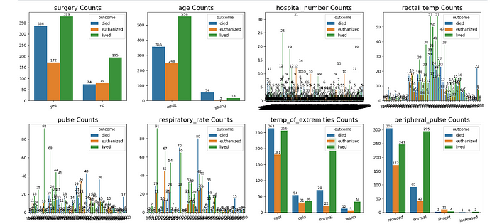
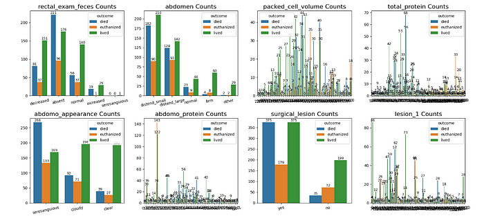
From the above plots, we can infer many insights. few of them are mentioned below.

• There are three categories of outcomes lived, died, and euthanized. As we can observe, the number of deaths and deaths are almost the same and high in cases, even surgeries are done as compared to not taking any surgery.
• The number of adult horses is more than the number of young horses, and therefore, the outcomes also proportion to their count of ages.
• There are more deaths of young horses percentage as we can observe from the plots.
• We can also observe horses' outcomes in different temperatures. As we can observe, there are more likely to live horses where the temperature is normal and cool, but in cool temperatures, there are more horses that are dead.
• We can also observe that as pulse count is normal and reduced ones are more horse and their lived and death ratios are almost similar and high as in reduced pulse counts and less in deaths in normal pulse counts.

Similarly, there are many other features that affect the prediction of the health of horses, as you can see in the plots below.

3. Data Pre-Processing

In the domain of machine learning, data cleaning stands as a pivotal step wherein we undertake various actions to ensure our dataset is free from anomalies, thereby facilitating the extraction of meaningful insights and enabling accurate predictions.

Handling Missing Values:

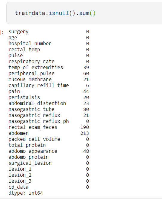
• Ensuring the absence of missing values in our dataset before model fitting is paramount for accurate predictions. It’s incumbent upon us to meticulously examine our data for null values and responsibly address them through techniques such as imputation or elimination.
• While dropping null values may impact the accuracy of our results, the decision hinges on factors such as the number of missing values and their significance in the dataset, thereby necessitating thoughtful consideration akin to feature engineering or selection in machine learning.

traindata.isnull().sum()

Encoding Categorical Variables:
Encoding categorical variables is a crucial pre-processing step in machine learning when working with datasets that contain non-numeric or categorical data.

Categorical variables represent qualitative characteristics or groups that do not have a natural ordering, such as colors, types of objects, or categories of data.
Feature Scaling:
Feature scaling is a pre-processing technique used in machine learning to standardize or normalize the range of independent variables or features in a dataset. It is particularly important when working with algorithms sensitive to the scale of input features.

The main goal of feature scaling is to bring all features to a similar scale without distorting the differences in the range of values. This helps in improving the performance and convergence of machine learning algorithms. Here I just considered numerical features for the first iteration.

numerical_features = []

for column in traindata.columns:
 
 if pd.api.types.is_numeric_dtype(traindata[column]):
 
 numerical_features.append(column)

features=numerical_features

xtrain=pd.get_dummies(xtrain)
xval=pd.get_dummies (xval)
print (xtrain.shape, xval.shape, ytrain.shape, yval.shape)

Data Splitting (Training and Validation):

• To design efficient ML models, we need to train the model on a particular portion of data and then will have to check how our designed model works on another data set, and that is what we call validation data.
• Training a model of one data and testing the model with the same data will give us a 100% accurate model, and that is a blender since we don’t know what kind of data we need to predict, so it is recommended to split our data into train and validation data for testing our model.

xtrain, xval, ytrain, yval = train_test_split(traindata[features], targetdata, test_size=0.1, random_state=1)
print (xtrain.shape, xval.shape, ytrain.shape, yval.shape)

4. Model Development & Model Evaluation

Algorithm Selection:

Algorithm selection is a crucial aspect of the machine learning workflow, involving the careful consideration and choice of the most appropriate algorithm for a given problem. This process is essential because different algorithms have varying strengths, weaknesses, and suitability for specific types of data and tasks.

Here’s some information about algorithm selection:

1. Understanding Algorithm Types: Machine learning algorithms can be broadly categorized into various types, such as supervised learning, unsupervised learning, and reinforcement learning. Within each type, there are further subcategories, including classification, regression, clustering, and dimensionality reduction algorithms.
2. Matching Algorithm to Task: The first step in algorithm selection is understanding the nature of the task at hand. For example, if the task involves predicting a categorical outcome, classification algorithms such as logistic regression, decision trees, or support vector machines may be suitable. If the task involves predicting a continuous outcome, regression algorithms like linear regression or random forests might be more appropriate.
3. Consideration of Data Characteristics: The characteristics of the dataset, such as size, complexity, and feature types, play a significant role in algorithm selection. Some algorithms are better suited for large datasets, while others perform well with high-dimensional data or data with non-linear relationships.
4. Performance Metrics: It’s essential to consider the performance metrics relevant to the task when selecting an algorithm. For example, if the goal is to minimize prediction errors, algorithms that optimize for accuracy, precision, recall, or F1 score may be preferred. In contrast, for unsupervised tasks like clustering, metrics such as silhouette score or Davies–Bouldin index may be used.
5. Model Interpretability: Depending on the application, the interpretability of the model may also be a crucial factor. Some algorithms, like decision trees or linear models, offer interpretability by providing insights into feature importance or coefficients. In contrast, other algorithms, such as neural networks or ensemble methods, may sacrifice interpretability for predictive performance.
6. Cross-Validation and Evaluation: Before finalizing the algorithm selection, it’s essential to perform thorough evaluation and validation using techniques like cross-validation to ensure the chosen algorithm generalizes well to unseen data and performs consistently across different subsets of the dataset.

In summary, algorithm selection involves a comprehensive assessment of the task requirements, data characteristics, performance metrics, and model interpretability to choose the most suitable algorithm that aligns with the objectives of the machine learning project.

Here I considered the Random forest algorithm for predictions.

model=RandomForestClassifier(n_estimators=100, max_depth=7, random_state=1 )

Model Training:
In this step we are going to train the model by fitting the train data to model and predict the results.

model=model.fit(xtrain, ytrain)
pred=model.predict(xval)

Model Evaluation Metrics:
Due to classification problems, we will check accuracy, precision, recall, and f1scores. Here it is asked to check especially f1score. So we will find f1score in this problem.

# precision = precision_score(yval, pred)
# recall = recall_score(yval, pred)
from sklearn.metrics import f1_score

# Assuming y_true and y_pred are your true and predicted labels
f1 = f1_score(yval, predi, average='micro')

testdata = pd.read_csv('/kaggle/input/playground-series-s3e22/test.csv')
testdf=testdata[features]
testdf.shape
testdf.isnull().sum()
testdf=pd.get_dummies(testdf)
modelpred=model.predict(testdf)
modelpred

mapping = {0: 'died', 1: 'euthanized', 2: 'lived'}

# Convert numerical labels to categorical labels
prediction = [mapping[i] for i in modelpred ]
prediction=np.array(prediction)

prediction=pd.DataFrame({'id': testdata['id'], 'outcome':prediction})
prediction.to_csv('submission1.csv', index=False)

This is the project series from the Kaggle playground series. Click Here to see the details on Kaggle.

Kindly support me by clapping or by giving feedback, which helps me to work on delivering quality content and gives me the motivation to move forward to share more content.

Thank you 🙂

Join thousands of data leaders on the AI newsletter. Join over 80,000 subscribers and keep up to date with the latest developments in AI. From research to projects and ideas. If you are building an AI startup, an AI-related product, or a service, we invite you to consider becoming a sponsor.

Published via Towards AI