Introduction to the Markov Chain, Process, and Hidden Markov Model

Last Updated on January 6, 2023 by Editorial Team

Author(s): Satsawat Natakarnkitkul

Data Science, Machine Learning

The concept and application of Markov chain and Hidden Markov Model in Quantitative Finance

Introduction

In the recent advancement of the machine learning field, we start to discuss reinforcement learning more and more. Reinforcement learning differs from supervised learning, where we should be very familiar with, in which they do not need the examples or labels to be presented. The focus of reinforcement learning is finding the right balance between exploration (new environment) and exploitation (use of existing knowledge).

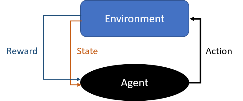
The environment of reinforcement learning generally describes in the form of the Markov decision process (MDP). Therefore, it would be a good idea for us to understand various Markov concepts; Markov chain, Markov process, and hidden Markov model (HMM).

Markov process and Markov chain

Both processes are important classes of stochastic processes. To put the stochastic process into simpler terms, imagine we have a bag of multi-colored balls, and we continue to pick the ball out of the bag without putting them back. In such a way, a stochastic process begins to exist with color for the random variable, but it does not satisfy the Markov property. Because each time the balls are removed, the probability of getting the next particular color ball may be drastically different. However, if we allow the balls to be put back into the bag, this creates a stochastic process with color for the random variable. However, this satisfies the Markov property.

With this in mind, the Markov chain is a stochastic process. However, the Markov chain must be memory-less, which is the future actions are not dependent upon the steps that lead up to the present state. This property is called the Markov property.

Knowledge of the previous state is all that is necessary to determine the probability distribution of the current state.

A Markov chain is a discrete-time process for which the future behavior only depends on the present and not the past state. Whereas the Markov process is the continuous-time version of a Markov chain.

Markov Chain

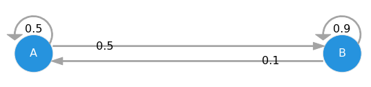
Markov chain is characterized by a set of states S and the transition probabilities, Pij, between each state. The matrix P with elements Pij is called the transition probability matrix of the Markov chain.

Note that the row sums of P are equal to 1. Under the condition that;

• All states of the Markov chain communicate with each other (possible to go from each state, in more than one step to every other state)
• The Markov chain is not periodic (periodic Markov chain is like you can only return to a state in an even number of steps)
• The Markov chain does not drift to infinity

Markov Process

The main difference is how the transition behavior behaves. In each state, there are a number of possible events that can cause a transition. The event that causes a transition from the state I to J, can take place after an exponential amount of time, Qij.

The system can make a transition from state i to state j with a probability of;

The matrix Q with elements of Qij is called the generator of the Markov process. The row sums of Q are 0. Under the conditions;

• All states of the Markov process communicate with each other
• The Markov process does not drift toward infinity

Application

We actually deal with Markov chain and Markov process use cases in our daily life, from shopping, activities, speech, fraud, and click-stream prediction.

Let’s observe how we can implement this in Python for loan default and paid up in the banking industry. We can observe and aggregate the performance of the portfolio (in this case, let’s assume we have 1-year data). We can compute the probability path, P(good loans -> bad loans) = 3%, and construct the transition matrix.

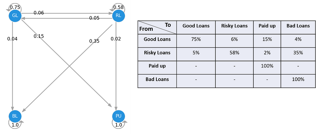
Once we have this transition, we can use this to predict how will the loan portfolio becomes at the end of year 1. Assuming we have two portfolios, one with 90% of a good loan and 10% of risky, and another with 50:50.

At the end of year one, port A will have 13.7% paid-up and 7.1% bad loans, while there’re 11.2% becomes risky loans. Port B will become 40%, 32%, 8.5%, and 19.5% of good loans, risky loans, paid-up, and bad loans, respectively.

Assumptions and Limitations of Markov Model

The Markov Chain can be powerful tools when modeling stochastic processes (i.e. ordering and CRM events). However, there are a few assumptions that should be met for this technique.

Assumption 1: The probabilities apply to all participants in the system

Assumption 2: The transition probabilities are constant over time

Assumption 3: The states are independent over time

Hidden Markov Model (HMM)

Hidden Markov Models (HMMs) are probabilistic models, it implies that the Markov Model underlying the data is hidden or unknown. More specifically, we only know observational data and not information about the states.

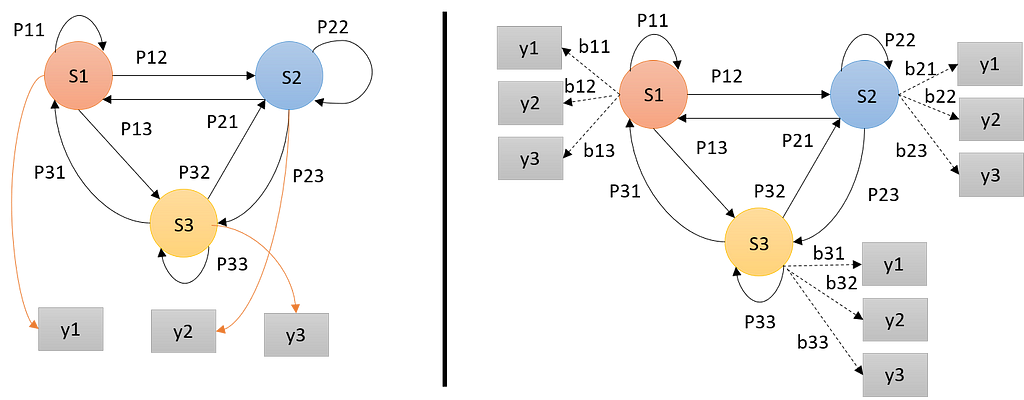
HMM is determined by three model parameters;

• The start probability; a vector containing the probability for the state of being the first state of the sequence.
• The state transition probabilities; a matrix consisting of the probabilities of transitioning from state Si to state Sj.
• The observation probability; the likelihood of a certain observation, y, if the model is in state Si.

HMMs can be used to solve four fundamental problems;

1. Given the model parameters and the observation sequence, estimate the most likely (hidden) state sequence, this is called a decoding problem.
2. Given the model parameters and observation sequence, find the probability of the observation sequence under the given model. This process involves a maximum likelihood estimate of the attributes, sometimes called an evaluation problem.
3. Given observation sequences, estimate the model parameters, this is called a training problem.
4. Estimate the observation sequences, y1, y2, …, and model parameters, which maximizes the probability of y. This is called a Learning or optimization problem.

Use case of HMM in quantitative finance

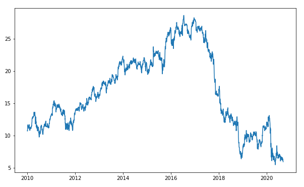
Considering the largest issue we face when trying to apply predictive techniques to asset returns is a non-stationary time series. In other words, the expected mean and volatility of asset returns changes over time. Most of the time series models and techniques assume that the data is stationary, which is the major weakness of these models.

Now, let’s frame this problem differently, we know that the time series exhibit temporary periods where the expected means and variances are stable through time. These periods or regimes can be associated with hidden states of HMM. Based on this assumption, all we need are observable variables whose behavior allows us to infer to the true hidden states.

In the finance world, if we can better estimate an asset’s most likely regime, including the associated means and variances, then our predictive models become more adaptable and will likely improve. Furthermore, we can use the estimated regime parameters for better scenario analysis.

In this example, I will use the observable variables, the Ted Spread, the 10-year — 2-year constant maturity spread, the 10-year — 3-month constant maturity spread, and ICE BofA US High Yield Index Total Return Index, to find the hidden states

In this example, the observable variables I use are the underlying asset returns, the ICE BofA US High Yield Index Total Return Index, the Ted Spread, the 10 year — 2-year constant maturity spread, and the 10 year — 3-month constant maturity spread.

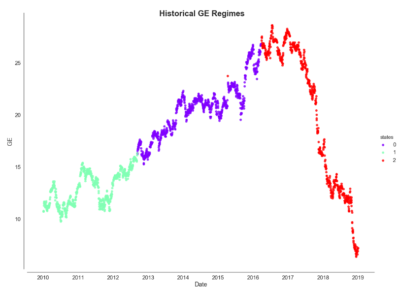
Now we are trying to model the hidden states of GE stock, by using two methods; sklearn's GaussianMixture and HMMLearn's GaussianHMM. Both models require us to specify the number of components to fit the time series, we can think of these components as regimes. For this specific example, I will assign three components and assume to be high, neural, and low volatility.

Gaussian Mixture method

This mixture models implement a closely related supervised form of density estimation by utilizing the expectation-maximization algorithm to estimate the mean and covariance of the hidden states. Please refer to this link for the full documentation.

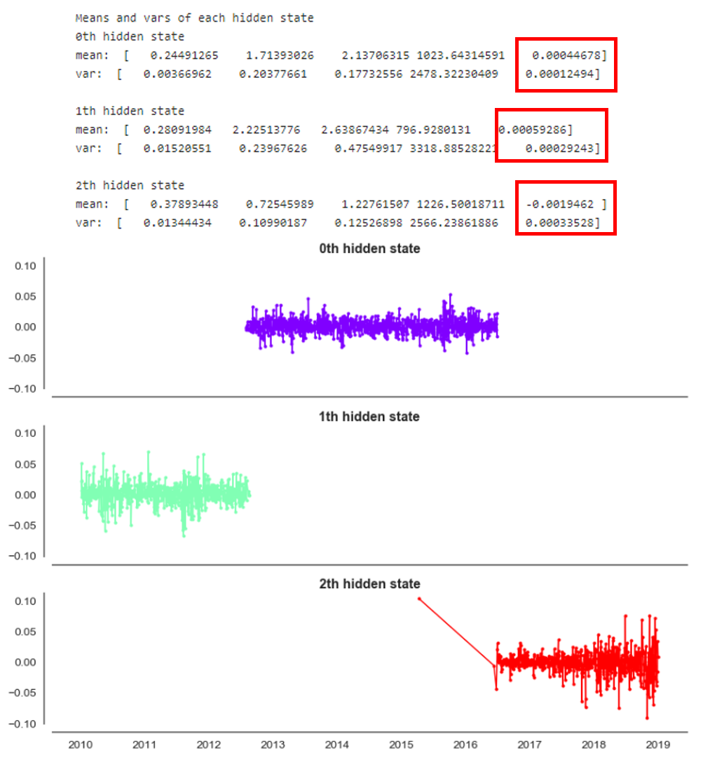
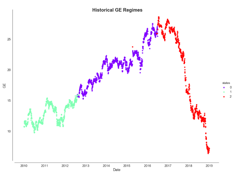
The red highlight indicates the mean and variance values of GE stock returns. We can interpret that the last hidden state represents the high volatility regime, based on the highest variance, with negative returns. While the 0th and 1st hidden states represent low and neutral volatility. This neutral volatility also shows the largest expected return. Let’s map this color code and plot against the actual GE stock price.

HMMLearn’s GaussianHMM

The HMMLearn implements simple algorithms and models to learn Hidden Markov Models. There are multiple models like Gaussian, Gaussian mixture, and multinomial, in this example, I will use GaussianHMM . For more details, please refer to this documentation.

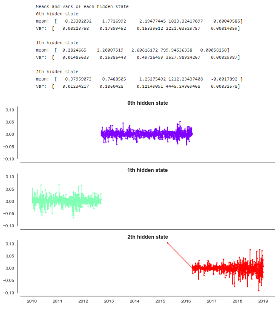
The result from GaussianHMM exhibits nearly the same as what we found using the Gaussian Mixture model.

Endnote

In this post, we have discussed the concept of Markov chain, Markov process, and Hidden Markov Models, and their implementations. We used the sklearn’s GaussianMixture and HMMLearn’s GaussianHMM to estimate historical regimes from other observation variables.

For the full code implementation, you can refer to here or visit my GitHub in the link below. Happy learning!!!

Reference and Github repository

Johns Hopkins Resource

• netsatsawat/markov_and_hidden_markov_model
• Towards AI – The Best of Tech, Science, and Engineering

---

Introduction to the Markov Chain, Process, and Hidden Markov Model was originally published in Towards AI — Multidisciplinary Science Journal on Medium, where people are continuing the conversation by highlighting and responding to this story.

Published via Towards AI