How Do Inherently Interpretable AI Models Work? — GAMINET

Author(s): Indraneel Dutta Baruah

Originally published on Towards AI.

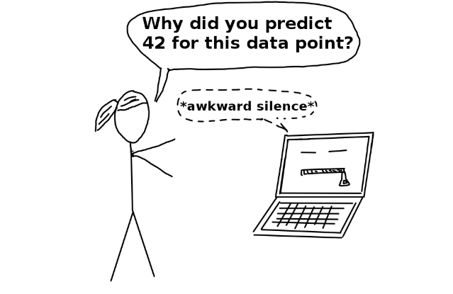
The field of deep learning has grown exponentially and the recent craze about ChatGPT is proof of the same. The models are becoming more and more complex with deeper layers leading to greater accuracy. One issue with this current trend is the focus on interpretability is lost at times. It is very risky to apply these black-box AI systems in real-life applications, especially in sectors like banking and healthcare. For example, a deep neural net used for a loan application scorecard might deny a customer, and we will not be able to explain why. This is where an explainable neural network based on generalized additive models with structured interactions (GAMI-Net) comes into the picture. It is one of the few deep learning models that are inherently interpretable.

If you are not aware of how neural networks work, it is highly advised that you brush on that first by going through this blog series.

So, without further ado, let’s dive in!

What is GAMINET?

GAMINET is a neural network that consists of multiple additive subnetworks. Each subnetwork consists of multiple hidden layers and is designed for capturing one main effect (direct impact of an input variable on a target variable) or one pairwise interaction (combined impact of multiple input variables on a target variable). These subnetworks are then additively combined to form the final output. GAMI-Net is formulated as follows:

where hj (xj ) are main effects and fjk(xj , xk) are interaction effects.

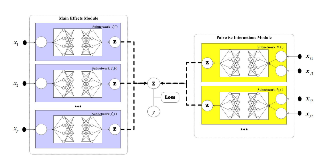
As shown in the figure above, Each main effect hj (xj ) is calculated by a subnetwork consisting of one input node using xj, numerous hidden layers, and one output node. Similarly, the pairwise interaction fjk(xj , xk) is calculated using a subnetwork with two input nodes (based on xj, xk). Finally, all the subnetworks are combined along with a bias term to predict the target variable.

Now that we know the overall structure of GAMINET, let’s discuss how certain constraints help make this model interpretable.

GAMINET Constraints

To improve the interpretability and identifiability of the impact of an input feature, GAMI-Net is developed with 3 constraints:

Sparsity constraint:

If we have a lot of input features, GAMI-net can end up having too many main and interaction effects. For example, if we have 100 input features, we will have 100 main effects and 4950 interaction effects! Thus, we need to keep only the critical effects for efficient computation and better interpretability. The importance of a main effect or pairwise interaction can be quantified based on the variance in the data explained by it. For example, the main effect of input feature xj can be measured as:

where n is the sample size. GAMI-Net picks the top s1 main effects ranked by D(hj ) values. s1 can be any user-defined number between 1 to the number of input features). Similarly, the top s2 pairwise interactions are picked using D(fjk):

Hereditary Constraint:

This constraint requires that a pairwise interaction can be included if at least one of its parent main effects is included by s1. This helps prune the number of interaction effects in the model.

Marginal Clarity

It can become difficult to quantify the impact of an input feature if the main effects are absorbed by their child interactions or vice versa. For example, if there are 3 variables x1, x2 and x3, f12(x1 , x2) and f12(x1 , x2) might absorb the impact of h(x1) itself. The marginal clarity constraint ensures such situations don’t occur by ensuring the impact of a feature can be uniquely decomposed into orthogonal components. This is similar to the functional ANOVA decomposition. Thus, marginal clarity constraints refer to the orthogonality condition for the j-th main effect and the corresponding pairwise interaction (j, k) as follows:

To learn more about orthogonal functions, you can go through this video.

Now we are ready to understand the model training process!

How does GAMI-net get trained?

The training process has the following three stages.

1. Training main effects: In this stage, the model trains all the main effect subnetworks for some epochs. It then removes the trivial main effects according to their variance contributions and validation performance
2. Training interaction effects: Train pairwise interaction effects that satisfy the hereditary constraint. Similar to the main effects, prune the weak pairwise interactions according to their variance contributions and validation performance
3. Fine-tune all the network parameters for some epochs

Let’s dive deep into each stage next.

Steps for training main effects:

Here are the main steps involved in training and identifying the main effects:

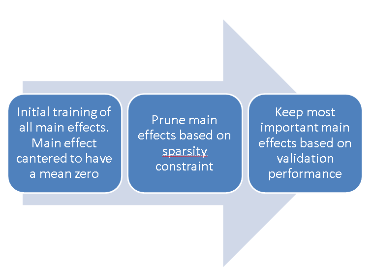
1. Main effect subnetworks are simultaneously estimated. The pairwise interaction subnetworks are set at zero in this stage. Mini-batch gradient descent is used for training along with Adam optimizer and adaptive learning rates.
2. The training continues till the maximum number of epochs or the validation accuracy doesn’t increase for some epochs
3. The main effect is centered on having a zero mean such that the bias in the output layer represents the mean of the target variable
4. The top main effects based on sparsity constraint are selected
5. The next step is to estimate the validation performance. Starting with a null model with just the intercept term, its validation set performance is recorded (say l0).
6. It is followed by adding the most important main effect based on the variance explained and its validation performance (say l1) is recorded. The other important main effects will be added in a sequence based on the variance explained and their validation performance is added to the list {l0, l1, · · · , lp}
7. The validation performance will start deteriorating when too many main effects are added due to overfitting training data. The final set of main effects (say S1) is set to the main effects whose validation loss is smaller than or equal to (1+η) min{l0, l1, · · · , lp}. η is a tolerance threshold added to make the model robust.

At this stage, we have the set of final main effects subnetworks S1. The next step is to identify the final pairwise interaction effects.

Steps for training interaction effects:

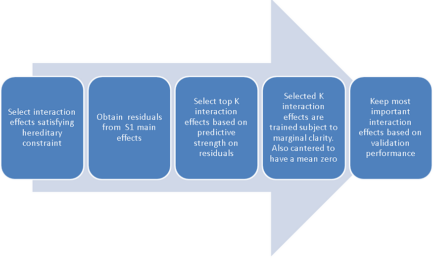
1. Identify interaction effects satisfying the hereditary constraint
2. Calculate the residuals from the final set of main effects (S1) subnetworks
3. For each j<k, with j ∈ S1 or k ∈ S1, shallow tree-like models using variables xj and xk are built (using the residuals from step 1 as the target variable)
4. The top K interaction effects are selected based on the minimum value of the loss function
5. The S1 main effect subnetworks are fixed, and top-K pairwise interactions are trained. Similar to the main effects, a minibatch gradient algorithm is used (but subject to marginal clarity regularization)
6. Again, similar to the main effects, the estimated pairwise interactions are centered to have zero mean.
7. Finally, the pruning method similar to the main effect is applied. First, a model with the intercept term and active main effects are trained and validation performance is noted( say t0). Then top-ranked pairwise interactions (based on the variance explained) are added one by one and validation performance is recorded {t0, t1,t2 · · · }.
8. The tolerance threshold η (same as the main effects) is used to balance predictive accuracy and interpretability. The final set of interaction effects (say S2) is set to those effects whose validation loss is smaller than or equal to (1+η) min{t0, t1,t2 · · · }

Steps for Fine Tuning:

1. Once both S1 main effects and S2 interaction effects are identified, GAMI-net jointly retrains all the active subnetworks, subject to marginal clarity regularization.
2. Similar to the previous steps, the main effects and pairwise interactions are re-centered to have zero mean.

This final step is performed to improve predictive performance as the initial interaction effect estimation was conditional on the pre-trained main effects.

Interpretability of GAMI-Net

There are three major methods to use for interpreting the model:

Importance Ratio (IR)

The importance of each input feature to the overall predictions of the model is calculated by the Importance Ratio (IR). For example, the IR for the main effect of input variable xj is calculated as:

where

Similarly, the IR of each pairwise interaction can be measured by:

It is important to note that the IR’s of all the effects sum up to one.

Global Interpretation

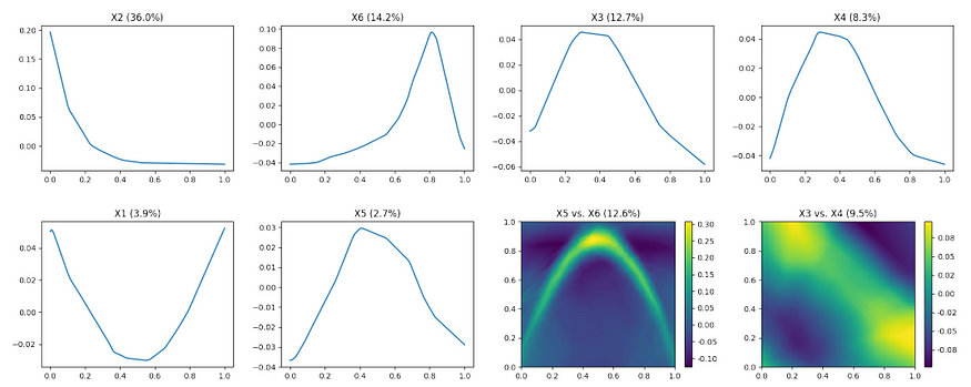
For inherently interpretable models like GAMI-net, the partial dependence relationships between input features and target variable (say y) can be directly calculated from the model equations. As shown in the figure above, 1D line plots can be calculated from hj (xj ) for j ∈ S1 for numeric features to show the relationship between an input feature and y. For the categorical features, bar charts can be used. For pairwise interaction, 2D heatmap can show the joint impact of two input features as seen in the figure above.

Local Interpretation

For each input data, GAMI-net can show us the exact function form as shown in Figure 1 earlier. The values of each additive subnetwork (both main and interaction) can be calculated and rank-ordered to understand how the prediction for a specific data point is made (see figure below).

What are the key hyperparameters?

The table below shows the list of important hyperparameters users should know about and their default values:

Conclusion

Thank you for reading my 4 part series on inherently interpretable AI models! The readers should now be able to understand the math behind four such models.

For several important real-world problems (especially in sectors like banking and healthcare), the focus on interpretability is here to stay. The current focus on interpretable AI has led to more advanced models like EBM and GAMI-net being developed, which use advanced models like neural nets and boosted trees while also informing how each prediction is made. I am hopeful that this trend will continue to grow and that we don’t have to face a trade-off between accuracy and interpretability.

In my next blog series, we will discuss the various Post hoc interpretation methods like SHAP, LIME, etc.

References

1. Original Paper:
   https://pdodds.w3.uvm.edu/files/papers/others/1986/hastie1986a.pdf
2. Gaminet Python Package Documentation: https://github.com/SelfExplainML/GamiNet
3. pyGAM Documentation: https://pygam.readthedocs.io/en/latest/notebooks/tour_of_pygam.html

Join thousands of data leaders on the AI newsletter. Join over 80,000 subscribers and keep up to date with the latest developments in AI. From research to projects and ideas. If you are building an AI startup, an AI-related product, or a service, we invite you to consider becoming a sponsor.

Published via Towards AI