Checking the Sentiment of a Tweet Using Machine Learning
Last Updated on July 24, 2023 by Editorial Team
Author(s): Saikat Biswas
Originally published on Towards AI.

Let’s see some tweets and classify them as positive or negative sentiment
When we hear the word Twitter, what does it ring to our ears? Well, for some, its a source of information where people get news in an instant, for some, it’s a place to voice their opinions and for some, it's just an app on their phone.
With the advent of smartphones since the last decade, Twitter has gradually made its shift from being a microblogging site that was originally launched as a replacement for SMS to being now shipped as an inbuilt app on our phones. Now, all of us have this app within our reach where we use it to check the news, follow publications, follow personalities and celebrities who have made it a customary part of their PR along with Instagram and Facebook to update on Twitter.
In short, If you are a hotshot, an update on Twitter means news.
Now since all of the major and small companies, trusts, institutions, movie premieres, an art or a boutique company, movie production houses, restaurants, the list goes on have their own Twitter handle, they often keep their followers posted with anything that they deem necessary for them to know via their handle.
And once they do, people often get inclined to voice their opinions, feelings, rants, disgusts and everything that they feel like venting it out on the platform.

And companies know this so they use Twitter to gauge the sentiment of the general public to know about their product launches and how they can improve upon their products further so that it reaches to wider sections of society which in turn would affect their businesses generating revenues.
We can see from the graph below that, all the contents of tweets on the Twitter world which is classified into various categories.

In my previous article, we saw how we check the sales of an item in a particular store using Machine Learning.
In this one, we will see how we can detect the sentiment of a particular tweet using Machine Learning.
Sentiment analysis remains one of the key problems that has seen an extensive application of natural language processing. We are given the tweets from customers about various tech firms who manufacture and sell mobiles, computers, laptops, etc, the task is to identify if the tweets have a negative sentiment towards such companies or products. We will work on this problem and then classify the tweets as a positive or negative sentiment.
For this purpose, we will go through a hackathon that is available on the AV platform and we will see how we can classify the tweets into various sentiments.
The complete code for this one can be found on my GitHub repo.
So, let’s get going.
We will divide the codes into 3 categories.
- EDA (Exploratory Data Analysis): Some Exploratory Analysis on the train and test data as a whole by combining them.
- Feature Engineering: Using the features for better prediction of sentiments.
- Modeling: The part where Machine Learning comes to the fore and we see the prediction results.
Enough talk. Show me the code..!!
# importing the libraries for data processing and analysis
import pandas as pd
import numpy as np
import matplotlib.pyplot as plt
import seaborn as sns
import warnings
%matplotlib inline
plt.style.use('fivethirtyeight')
warnings.filterwarnings('ignore')
Once this is done, we will proceed with loading the train and the test data.
train = pd.read_csv('train_sentiment.csv')
test = pd.read_csv('test_sentiment.csv')
- EDA (Exploratory Data Analysis)
We can check for the distribution of tweet counts in the train and test data.
# checking the distribution of label of tweets in the dataset
train[train['label'] == 0].head(10)
train[train['label'] == 1].head(10)
Next, we proceed with Count Vectorization of the tweet data. Count vectorization is the process of counting the number of occurrences of each word that appears in a document (i.e distinct text such as an article, book, even a paragraph!).
# count vectorization for the text
from sklearn.feature_extraction.text import CountVectorizer

cv = CountVectorizer(stop_words = 'english')
words = cv.fit_transform(train.tweet)

sum_words = words.sum(axis=0)

words_freq = [(word, sum_words[0, i]) for word, i in cv.vocabulary_.items()]
words_freq = sorted(words_freq, key = lambda x: x[1], reverse = True)

frequency = pd.DataFrame(words_freq, columns=['word', 'freq'])

frequency.head(30).plot(x='word', y='freq', kind='bar', figsize=(15, 7), color = 'brown')
plt.title("Most Frequently Occuring Words - Top 30")
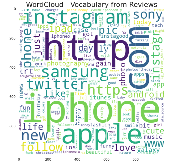
Another important EDA step that should proceed with is checking the most important words present in the data. So, generating a word cloud for the most occurring words present in the train data.
# generating word cloud for the most common occuring words in the train data
from wordcloud import WordCloud

wordcloud = WordCloud(background_color = 'white', width = 1000, height = 1000).generate_from_frequencies(dict(words_freq))

plt.figure(figsize=(10,8))
plt.imshow(wordcloud)
plt.title("WordCloud - Vocabulary from Reviews", fontsize = 22)
Let’s also check for the neutral words present in the tweet data.
# wordcloud for words that are neutral
normal_words =' '.join([text for text in train['tweet'][train['label'] == 0]])

wordcloud = WordCloud(width=800, height=500, random_state = 0, max_font_size = 110).generate(normal_words)
plt.figure(figsize=(10, 7))
plt.imshow(wordcloud, interpolation="bilinear")
plt.axis('off')
plt.title('The Neutral Words')
plt.show()

To check for the hashtags present in the data I created a function that checks and collects the hashtags present in the data and stores them in a list.
- We can also see the most important hashtags present in the tweet data.
- We can also check for the tweets type and store them in a list.
# defining a function to collect the hashtags from the train data
def hashtags_extract(x):
 hashtags = []
 for i in x:
 ht = re.findall(r"#(\w+)", i)
 hashtags.append(ht)

 return hashtags
#extracting hashtags from racist/sexist tweet
ht_normal = hashtags_extract(train['tweet'][train['label'] == 0])

#extracting hashtags from normal tweet
ht_negetive = hashtags_extract(train['tweet'][train['label'] == 1])

#unnesting list

ht_normal = sum(ht_normal , [])
ht_negetive = sum(ht_negetive , [])
Once that is taken care of, we proceed with tokenizing the words present in the data. Tokenization is an important step in NLP as it helps in breaking the words to its root form.
Post tokenization we create a word to vector model using the popular Gensim library keeping the context window size at 5 and window size at 1 for the skip-gram model.
#tokenizing the words present in the training set
tokenized_tweet = train['tweet'].apply(lambda x: x.split())

# importing gensim
import gensim

# creating a word to vector model
model_w2v = gensim.models.Word2Vec(
 tokenized_tweet,
 size=200, # desired no. of features/independent variables
 window=5, # context window size
 min_count=2,
 sg = 1, # 1 for skip-gram model
 hs = 0,
 negative = 10, # for negative sampling
 workers= 2, # no.of cores
 seed = 34)

model_w2v.train(tokenized_tweet, total_examples= len(train['tweet']), epochs=20)
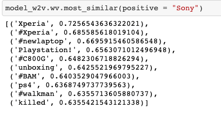
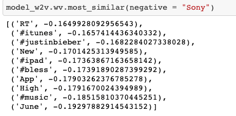
Once that is done we can see for ourselves the words that; have a meaning similar to the words present in the dataset. For eg:- “Sony”
from tqdm import tqdm
tqdm.pandas(desc="progress-bar")
from gensim.models.doc2vec import LabeledSentence# Adding a label to the tweetsdef add_label(twt):
 output = []
 for i, s in zip(twt.index, twt):
 output.append(LabeledSentence(s, ["tweet_" + str(i)]))
 return output

# label all the tweets
labeled_tweets = add_label(tokenized_tweet)

labeled_tweets[:6]
We should remove unwanted patterns from the data too as keeping them adds noise to our dataset and we should try to keep our model noise-free as much as possible for better prediction.
# removing unwanted patterns from the data

import re
import nltk

nltk.download('stopwords')
from nltk.corpus import stopwords
from nltk.stem.porter import PorterStemmer# collecting the train data and forming a corpus
train_corpus = []

for i in range(0, 7920):
 review = re.sub('[^a-zA-Z]', ' ', train['tweet'][i])
 review = review.lower()
 review = review.split()

 ps = PorterStemmer()
 # stemming
 review = [ps.stem(word) for word in review if not word in set(stopwords.words('english'))]

 # joining them back with space
 review = ' '.join(review)
 train_corpus.append(review)
from sklearn.feature_extraction.text import CountVectorizer

cv = CountVectorizer(max_features = 1500)
x = cv.fit_transform(train_corpus).toarray()
y = train.iloc[:, 1]

print(x.shape)
print(y.shape)# creating bag of words for test

from sklearn.feature_extraction.text import CountVectorizer

cv = CountVectorizer(max_features = 1500)
x_test = cv.fit_transform(test_corpus).toarray()
y = train.iloc[:, 1]

print(x_test.shape)
Now, doing the same for the test data as well.
test_corpus = []

for i in range(0, 1953):
 review = re.sub('[^a-zA-Z]', ' ', test['tweet'][i])
 review = review.lower()
 review = review.split()

 ps = PorterStemmer()

 # stemming
 review = [ps.stem(word) for word in review if not word in set(stopwords.words('english'))]

 # joining them back with space
 review = ' '.join(review)
 test_corpus.append(review)
Removal of stopwords & lemmatization(Lemmatization, unlike Stemming, reduces the inflected words properly ensuring that the root word belongs to the language. In Lemmatization root word is called Lemma. A lemma (plural lemmas or lemmata) is the canonical form, dictionary form, or citation form of a set of words.) is also an important step when it comes to the processing of the Natural language.
# removing unwanted patterns from the data

import re
import nltk

nltk.download('stopwords')
from nltk.corpus import stopwords
from nltk.stem.porter import PorterStemmer# for train data
train_corpus = []

for i in range(0, 7920):
 review = re.sub('[^a-zA-Z]', ' ', train['tweet'][i])
 review = review.lower()
 review = review.split()

 ps = PorterStemmer()
 # stemming
 review = [ps.stem(word) for word in review if not word in set(stopwords.words('english'))]

 # joining them back with space
 review = ' '.join(review)
 train_corpus.append(review)# for test data
test_corpus = []

for i in range(0, 1953):
 review = re.sub('[^a-zA-Z]', ' ', test['tweet'][i])
 review = review.lower()
 review = review.split()

 ps = PorterStemmer()

 # stemming
 review = [ps.stem(word) for word in review if not word in set(stopwords.words('english'))]

 # joining them back with space
 review = ' '.join(review)
 test_corpus.append(review)
Now, we are almost done with the cleaning of the data and then we will create a bag of words by converting the words present in the corpus to an array for the machine to understand and process the data.
# creating bag of words for train
# creating bag of words

from sklearn.feature_extraction.text import CountVectorizer

cv = CountVectorizer(max_features = 1500)
x = cv.fit_transform(train_corpus).toarray()
y = train.iloc[:, 1]

print(x.shape)
print(y.shape)-------
(7920, 1500)
(7920,)# creating bag of words for test

from sklearn.feature_extraction.text import CountVectorizer

cv = CountVectorizer(max_features = 1500)
x_test = cv.fit_transform(test_corpus).toarray()
y = train.iloc[:, 1]

print(x_test.shape)-------
(1953, 1500)
# standardization

from sklearn.preprocessing import StandardScaler

sc = StandardScaler()

x_train = sc.fit_transform(x_train)
x_valid = sc.transform(x_valid)
Standardization is also an important step before we proceed with the modeling process.
Post Standardization, we split the data for train and test purposes.
from sklearn.model_selection import train_test_split

x_train, x_valid, y_train, y_valid = train_test_split(x, y, test_size = 0.25, random_state = 42)

print(x_train.shape)
print(x_valid.shape)
print(y_train.shape)
print(y_valid.shape)---------------
(5940, 1500)
(1980, 1500)
(5940,)
(1980,)
The Evaluation metric used for this competition is F1 Score which is formulated as 2*((precision*recall)/(precision+recall)).

Once we are done with this, we will proceed with Machine Learning modeling.
Let’s try a few Modelling techniques on the data and see the result for ourselves.
- Random Forest
from sklearn.ensemble import RandomForestClassifier
from sklearn.metrics import confusion_matrix
from sklearn.metrics import f1_score

model = RandomForestClassifier()
model.fit(x_train, y_train)

y_pred = model.predict(x_valid)

print("Training Accuracy :", model.score(x_train, y_train))
print("Validation Accuracy :", model.score(x_valid, y_valid))

# calculating the f1 score for the validation set
print("F1 score :", f1_score(y_valid, y_pred))---------------
Training Accuracy : 0.9994949494949495
Validation Accuracy : 0.8853535353535353
F1 score : 0.7926940639269406---------------

# confusion matrix
cm = confusion_matrix(y_valid, y_pred)
print(cm)---------------
[[1319 120]
 [ 107 434]]
2. Decision tree Classifier
from sklearn.tree import DecisionTreeClassifier

model = DecisionTreeClassifier()
model.fit(x_train, y_train)

y_pred = model.predict(x_valid)

print("Training Accuracy :", model.score(x_train, y_train))
print("Validation Accuracy :", model.score(x_valid, y_valid))

# calculating the f1 score for the validation set
print("f1 score :", f1_score(y_valid, y_pred))

# confusion matrix
cm = confusion_matrix(y_valid, y_pred)
print(cm)
----------------Training Accuracy : 0.9994949494949495
Validation Accuracy : 0.8378787878787879
f1 score : 0.700280112044818[[1284 155]
 [ 166 375]]
3. SVM Modelling
# trying SVC algorithm on the data
from sklearn.svm import SVC

model = SVC()
model.fit(x_train, y_train)

y_pred = model.predict(x_valid)

print("Training Accuracy :", model.score(x_train, y_train))
print("Validation Accuracy :", model.score(x_valid, y_valid))

# calculating the f1 score for the validation set
print("f1 score :", f1_score(y_valid, y_pred))

# confusion matrix
cm = confusion_matrix(y_valid, y_pred)
print(cm)----------------Training Accuracy : 0.9644781144781145
Validation Accuracy : 0.8621212121212121
f1 score : 0.7222787385554426
[[1352 87]
 [ 186 355]]
4. XG Boost Classifier
# trying xgboost classifier on the data
from xgboost import XGBClassifier

model = XGBClassifier()
model.fit(x_train, y_train)

y_pred = model.predict(x_valid)

print("Training Accuracy :", model.score(x_train, y_train))
print("Validation Accuracy :", model.score(x_valid, y_valid))

# calculating the f1 score for the validation set
print("f1 score :", f1_score(y_valid, y_pred))

# confusion matrix
cm = confusion_matrix(y_valid, y_pred)
print(cm)-------------------Training Accuracy : 0.8882154882154882
Validation Accuracy : 0.8792929292929293
f1 score : 0.7912663755458514
[[1288 151]
 [ 88 453]]
5. Logistic Regression
from sklearn.linear_model import LogisticRegression

model = LogisticRegression()
model.fit(x_train, y_train)

y_pred = model.predict(x_valid)

print("Training Accuracy :", model.score(x_train, y_train))
print("Validation Accuracy :", model.score(x_valid, y_valid))

# calculating the f1 score for the validation set
print("f1 score :", f1_score(y_valid, y_pred))

# confusion matrix
cm = confusion_matrix(y_valid, y_pred)
print(cm)----------------Training Accuracy : 0.9757575757575757
Validation Accuracy : 0.8323232323232324
f1 score : 0.6897196261682242
[[1279 160]
 [ 172 369]]
So, after using 5 algorithms on the train data and testing the same on the test data we can fairly come to a conclusion that Random Forest algorithm has yielded the highest accuracy amongst all the remaining algorithms, which has successfully classified the tweets as positive and negative with an accuracy of 79.2%.

Conclusion
Twitter has become an indispensable part of our lives for most of us now. A single tweet has the capacity to affect the sales of a product of a company or wreak havoc within the twitter community if the tweet goes viral I mean and people keep posting all kinds of tweets full of various sentiments every time. So, as Data Scientists we should be able to decipher the negative sentiment attached to a tweet to a positive one, that in turn is used by companies to gauge the effectiveness of a product launch or a marketing advertisement.
In future, such need to classify sentiments would rise much fold as more and more people are becoming tech-savvy.
And this is an opportunity for companies to go ahead of their competition by gauging the responses on their product reviews to gain further revenues in the ever-increasingly competitive market.
So, that all in this one. Until next time. Ciao..!!!
Join thousands of data leaders on the AI newsletter. Join over 80,000 subscribers and keep up to date with the latest developments in AI. From research to projects and ideas. If you are building an AI startup, an AI-related product, or a service, we invite you to consider becoming a sponsor.
Published via Towards AI
Towards AI Academy
We Build Enterprise-Grade AI. We'll Teach You to Master It Too.
15 engineers. 100,000+ students. Towards AI Academy teaches what actually survives production.
Start free — no commitment:
→ 6-Day Agentic AI Engineering Email Guide — one practical lesson per day
→ Agents Architecture Cheatsheet — 3 years of architecture decisions in 6 pages
Our courses:
→ AI Engineering Certification — 90+ lessons from project selection to deployed product. The most comprehensive practical LLM course out there.
→ Agent Engineering Course — Hands on with production agent architectures, memory, routing, and eval frameworks — built from real enterprise engagements.
→ AI for Work — Understand, evaluate, and apply AI for complex work tasks.
Note: Article content contains the views of the contributing authors and not Towards AI.


