What is Overfitting and How to Solve It?

Author(s): Ibrahim Israfilov

Originally published on Towards AI the World’s Leading AI and Technology News and Media Company. If you are building an AI-related product or service, we invite you to consider becoming an AI sponsor. At Towards AI, we help scale AI and technology startups. Let us help you unleash your technology to the masses.

How to Solve Overfitting?

Theory of techniques used to overcome the overfitting

Introduction

As an econometrician or a data scientist, your task is to develop robust models and you need to master the regression (I love how J.Angrist says it) and how to regularize it.
For instance, for linear models, although linear regression is a golden standard for modeling, it might be not the best solution in certain circumstances. To keep it short, if your model is too complex for the underlying data which requires a simple model we are facing overfitting!

Overfitting and How to Solve It?

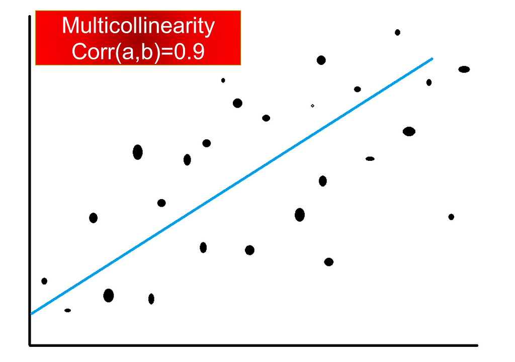
Overfitting is dangerous because of its sensibility when the model is putting too much weight on variance for the change as a result our model is overreacting to even the slightest change in our dataset. In data science and machine learning, this overreaction of our model is called overfitting. In linear models, whenever you have features that are highly correlated with other features (multicollinearity) your model is likely to overfit.
To avoid this to happen, you need to use a technique which is called a regularization (“shrinkage”) of coefficients for making the model be robust. In other words, you need to regularize your model by decreasing the pushing the coefficients of the estimated coefficients towards zero.
This technique in data science is called also a “Penalization of the regression”.
There are several ways of using this technique depending on the circumstances. We will see today Ridge Regression, Smoothing Splines, Local Regressions, and Lowess (Locally Weighted Regressions).

Ridge Regression

Is one of the often-used models in econometrics, engineering, etc. The regression is usually used when in the linear regression there has been observed the multicollinearity (high correlation) between independent variables.

The RR has less variance than OLS (which is usually unbiased) and stimulates the model to be more robust to the changes.

On the formula above λ≥0 is a tuning parameter that actually penalizes the regression to reduce the complexity.

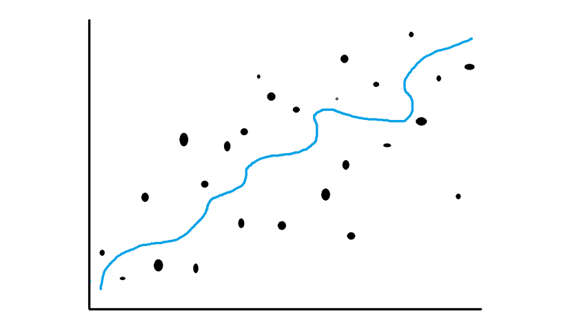
Smoothing Splines

When we talk about smoothing splines we are referring to non-linear models (For instance polynomial). Also, non-linear models suffer from overfitting when the model is too complex.

In this case, we will use the penalty for complexity as in ridge regression and what our formula is going to look like.

As you have already noticed it is similar to the RR model the only difference is the function of the predicted variable which in RR is β0+β1X1+β2X2+e. In our case, g(x) can be any other non-linear function which brings us to the overfitting (It is usually polynomial). λ is a smoothing effect. The larger λ the smoother the function g(x).

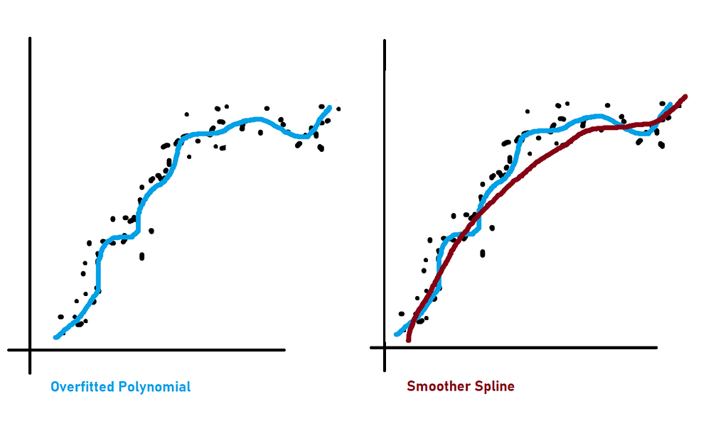
As you see the smoother spline model is prediction optimized.

Locally Weighted Regression (LOWESS)

The main idea behind this technique is to use the KNN regression within each neighborhood. This technique also contributes to the robustness of a model. The neighbors in KNN are found through Euclidian distance (But it’s not our topic today)

Local Regression (LOESS)

Loess is a powerful technique that can be used either with linear or non-linear Least Square regressions. LOESS is a non-parametric method so it doesn’t have a fixed formula. However, in order to compute the LOESS for X=x0, you need to follow the next steps.

• Gather the s= k/n of training data which Xi are closest to X0
• Assign a weight Ki0=K(xi,x0) where the nearest neighbor gets a certain weight and the furthest gets zero. All points beyond these neighbors are getting weight zero.
• Fit the weighted least squares regression

• The fitted value at x0 is given by

---

Machine Learning was originally published in Towards AI on Medium, where people are continuing the conversation by highlighting and responding to this story.

Join thousands of data leaders on the AI newsletter. It’s free, we don’t spam, and we never share your email address. Keep up to date with the latest work in AI. From research to projects and ideas. If you are building an AI startup, an AI-related product, or a service, we invite you to consider becoming a sponsor.

Published via Towards AI