


Author(s): Saniya Parveez
Machine Learning
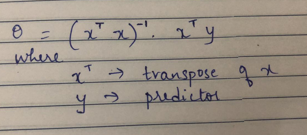
Gradient descent is a very popular and first-order iterative optimization algorithm for finding a local minimum over a differential function. Similarly, the Normal Equation is another way of doing minimization. It does minimization without restoring to an iterative algorithm. Normal Equation method minimizes J by explicitly taking its derivatives concerning theta j and setting them to zero.
Example:
Below is a data-set to predict house price:

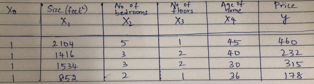
House Features:

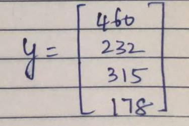
Predictor:

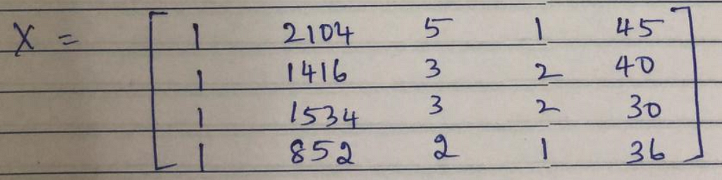
Calculation:
import numpy as np
x = np.array([[1, 2104, 5, 1, 45],
        [1, 1416, 3, 2, 40],
        [1, 1534, 3, 2, 30],
        [1, 852, 2, 1, 36]])
y = [460, 232, 315, 178]
x_transpose = x.transpose()
x_transpose_x = np.dot(x_transpose, x)
x_transpose_y = np.dot(x_transpose, y)
theta = np.dot(x_transpose_x_inverse, x_transpose_y)
theta
Gradient Descent Vs Normal Equation
Gradient Descent
- It requires to choose the value of Alpha.
- It requires many iterations.
- It works well when n (no. of data-set) is large.
Normal Equation
- It does not need to choose the value of Alpha.
- It doesn’t require iteration.
- It requires to calculate the inverse of transpose of x.
- It is slow if n (data-set) if very large.
Linear Regression with Normal Equation
Import libraries:
from numpy import genfromtxt
import numpy as np
from matplotlib import pyplot as plt
from sklearn.model_selection import train_test_split
from sklearn import linear_modl
Load the Portland data
data = genfromtxt('portland.csv', delimiter=',')
area = data[:, 0]
rooms =data[:, 1]
price = data[:, 2]
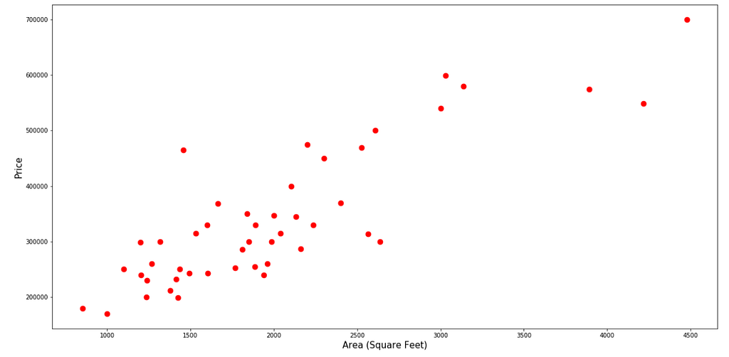
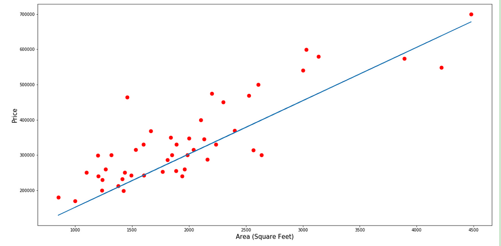
Visualize The Area against the Price:
def fitTheta(feature, theta):
return np.dot(theta, feature)
def visualiseFeature(feature, featureLabel, thetaVal=None):
fig = plt.figure(figsize=(20, 10))

    plt.rcParams.update({'font.size': 10})

    plt.xlabel(featureLabel, fontsize=15)

    plt.ylabel("Price", fontsize=15)

    plt.scatter(feature, price, color="red", s=75)

    if(thetaVal):

        thetaFit = fitTheta(feature, thetaVal)

        plt.plot(feature, thetaFit)

Visualize the Number of Rooms against the Price of the House:
visualiseFeature(rooms, "Number of Rooms")

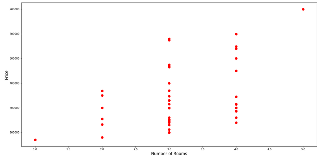
Here, the relationship between the Number of Rooms, and the Price of the House, appears to be Linear.
Define Feature Matrix, and Outcome/Target Vector:
X_data = data[:, 0:2] #Feature Matrix
y = data[:, 2] #Outcome Vector
Calculate Cost Function:
def getMSE(feature, thetaRange):
    costMatrix = np.repeat(price, thetaRange.shape[0]).reshape(price.shape[0], thetaRange.shape[0])

    costs = np.dot(np.asmatrix(feature).T, np.asmatrix(thetaRange)) - costMatrix

    MSE = (np.array((np.sum(costs, 0)))**2)/(2*price.shape[0])

    return np.array(MSE)[0]
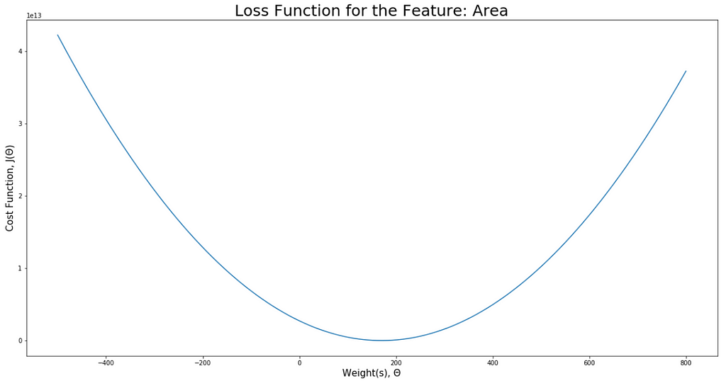
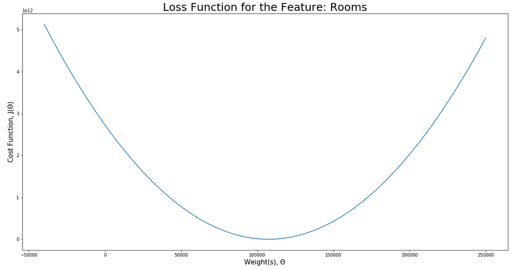
Visualize Cost Function:
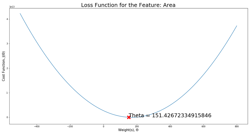
def visualiseLoss(feature, featureName, startInterval, endInterval, stepSize=0.5, thetaVal=None):
    thetaRange = np.arange(startInterval, endInterval, stepSize)

    Loss = getMSE(feature, thetaRange)

    fig = plt.figure(figsize=(20, 10))

    plt.title("Loss Function for the Feature: {}".format(featureName), fontsize=25)

    plt.ylabel("Cost Function, J(Θ)", fontsize=15)

    plt.xlabel("Weight(s), Θ", fontsize=15)

    plt.plot(thetaRange, Loss, zorder=1)

    if(thetaVal):

        thetaLoss = getMSE(feature, np.array(thetaVal).reshape(1, 1))

        plt.scatter(thetaVal, thetaLoss, marker="x", linewidth=5, color="red", s=200, zorder=2)

        plt.annotate("Theta = {}".format(thetaVal), (thetaVal, thetaLoss), fontsize=25)
visualiseLoss(area, "Area", -500, 800)
Add alt text

visualiseLoss(rooms, "Rooms", -40000, 250000)

Split Data
X_data = data[:, 0:2] #Feature Matrix
y = data[:, 2] #Outcome Vector
X = np.c_[np.ones(X_data.shape[0]), X_data]
X_train, X_test, y_train, y_test = train_test_split(X, y, test_size=0.2)
Normal Equation
firstTerm = np.linalg.inv(np.dot(X_train.T, X_train))
secondTerm = np.dot(X_train.T, y_train)
Theta = np.dot(firstTerm, secondTerm)
Visualize:
visualiseLoss(area, "Area", -500, 800, thetaVal=Theta[1])

visualiseFeature(area, "Area (Square Feet)", thetaVal=Theta[1])
Add alt text

Prediction using Normal Equation theta value
normal_predictions = np.dot(X_test, Theta)
normal_predictions
Add alt text


Prediction using Linear Regression
reg = linear_model.LinearRegression()
reg.fit(X_train, y_train)
sk_predictions = reg.predict(X_test)
sk_predictions
Add alt text


Here, the predictions from the Normal Equation and Linear Equation are the same.
Normal Equation Non-Invertibility
A squared matrix that does not have an inverse a matrix is singular if and only if it is determined is zero.
Example:
import numpy as np
A = [[2, 6],
[1, 3]]
The inverse of Matrix:
inverse_A = np.linalg.inv(A)
inverse_A
Error from Numpy:
Add alt text

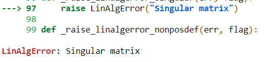
Problem due to Non-Invertibility:
- Redundant features
- Too many features
How to solve if there are too many features?
- Delete some features of use Regularization
Conclusion
Gradient Descent gives one way to minimizing J. Normal Equation is another way of doing minimization. It does minimization without restoring to an iterative algorithm. But, Normal Equation is very slow if the data-set size is very large

Normal Equation in Linear Regression was originally published in Towards AI — Multidisciplinary Science Journal on Medium, where people are continuing the conversation by highlighting and responding to this story.
Published via Towards AI