Logo:
Logo:  Areas Served:
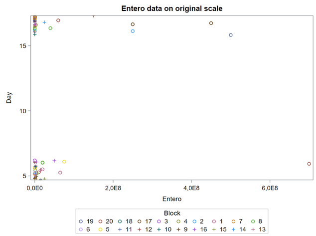
Using PROC GLIMMIX in SAS — examples
Last Updated on March 24, 2022 by Editorial Team
Author(s): Dr. Marc Jacobs
Originally published on Towards AI the World’s Leading AI and Technology News and Media Company. If you are building an AI-related product or service, we invite you to consider becoming an AI sponsor. At Towards AI, we help scale AI and technology startups. Let us help you unleash your technology to the masses.
Analyzing non-normal data in SAS — log data, mortality, litter, and preference scores.
This post is the last in a series showing the potential of PROC GLIMMIX which is the de facto tool for using Generalized Linear Mixed Models. After an introductory post and showing examples using the Multinomial, Binary, Binomial, Beta, Poisson, and Negative Binomial it is now time to go deeper into situations often encountered when analyzing data in the animal sciences. To be more precise, I will show examples of bacterial counts, litter scores, mortality scores, and preference scores. Enjoy!
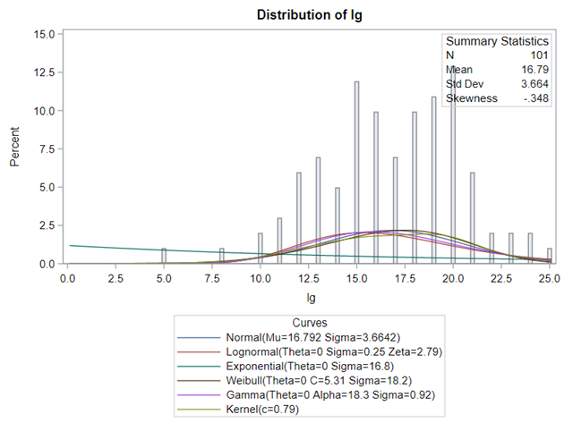
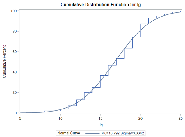
First of, bacterial counts and how to analyze data on the log scale. Data that have such a wide distribution that they need to be analyzed using a log scale can be surprisingly difficult to model inside a GLIMMIX model, especially when you use the log function. I will show you later what I mean.
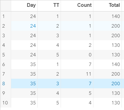
Below you see entero data on two points — five and fifteen — across their blocks in a Randomized Complete Block Design.
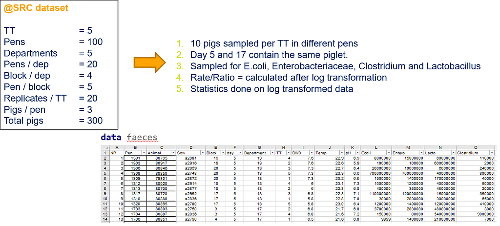
Below you can see the datasets used. This was a nested design having data across departments, blocks, and pens.
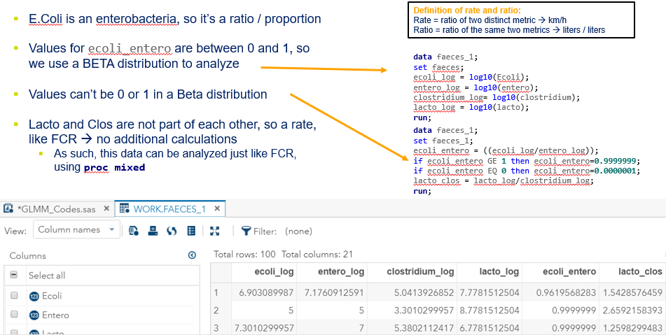
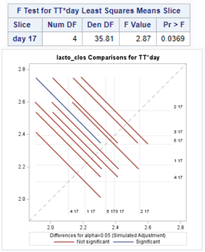
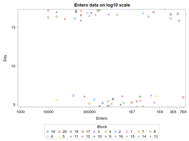
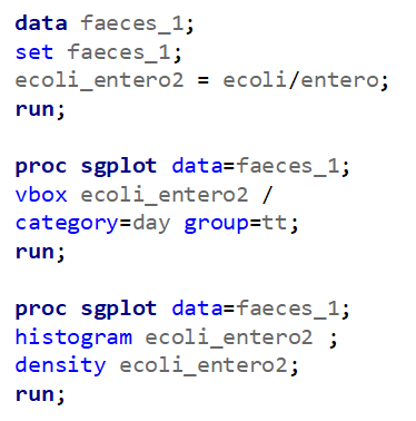
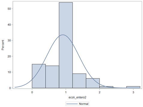
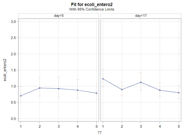
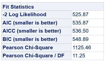
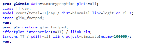
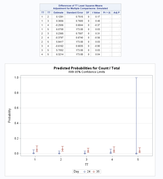
The above looked quite straightforward. A different song will be sung when you analyze the E.coli/Entero rate. Two straightforward plots down below easily indicate that you are dealing with a rate that is moving at the boundary of space.
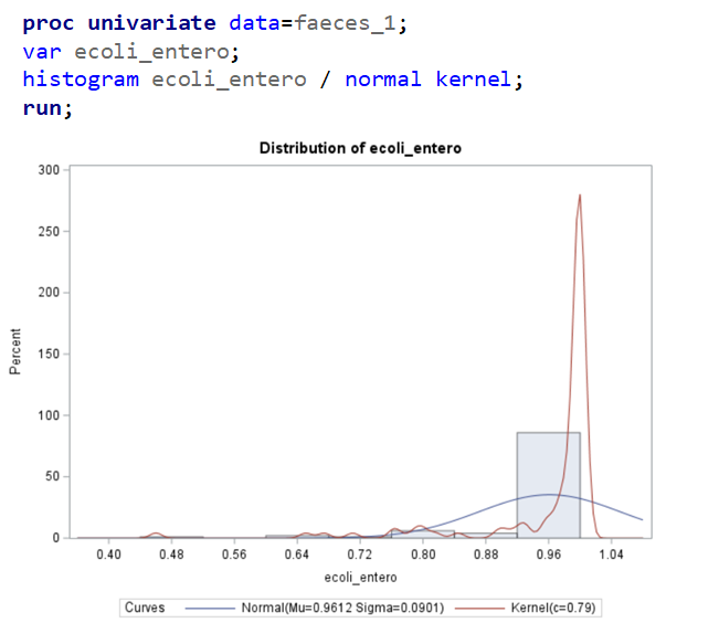
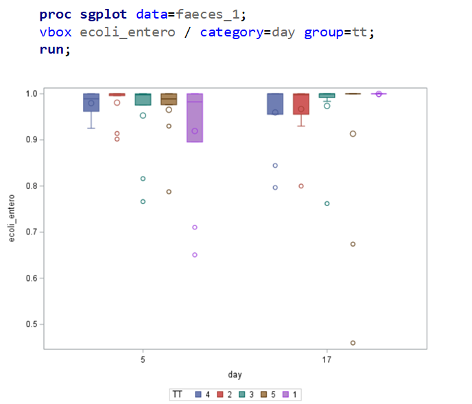
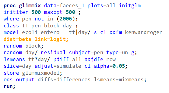
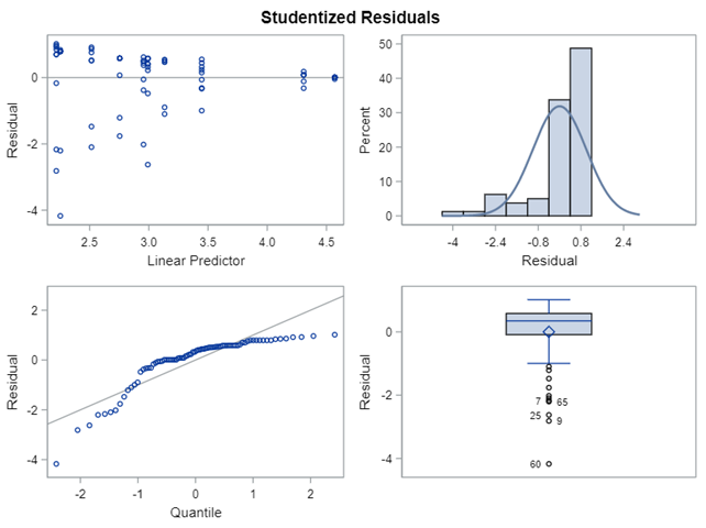
The problem in this example is not the distribution, but the data. The way the data is set up produces a strange rate that cannot be mimicked by the majority of the known distributions. Of course, a mixture distribution could be used, but what about changing the rate?
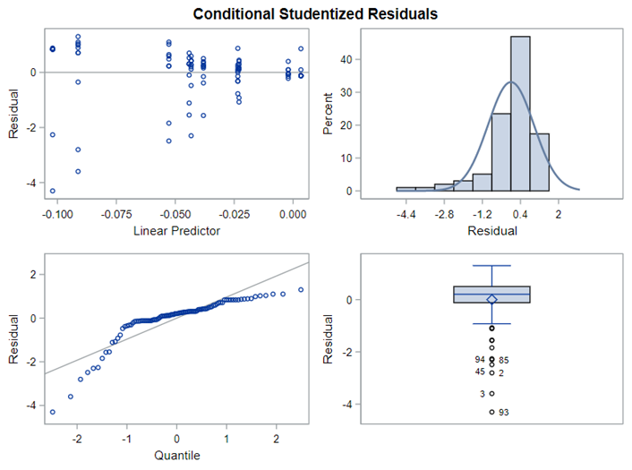
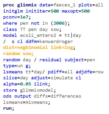
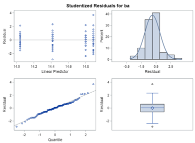
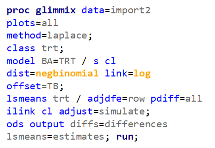
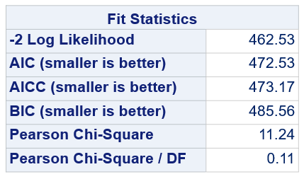
So, that is what I did. I changed the rate by using the raw data, and not the log scales. If you plot this rate, it looks much more Normal. As such, the Negative Binomial will have no problem modeling it.


In summary, I showed the analysis of four different variables, on the log scale, which we then combined into two new variables:
- a ratio of E.Coli and Enterobacteriaceae
- a rate of Clostridium and Lactobacillus
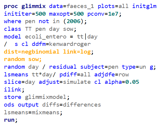
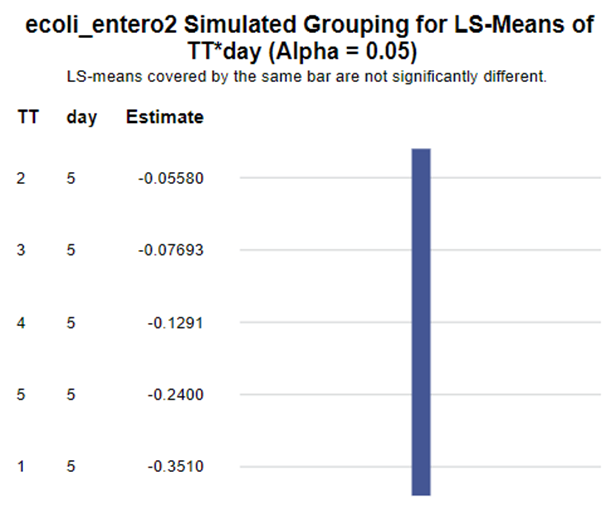
The ratio of Lactobacillus/Clostridium can be analyzed like the FCR in PROC Mixed. The rate of log(E.Coli) / log(Enterobacteriaceae) presents problems that are more difficult to overcome — distribution is difficult to model. Best to use E.Coli / Enterobacteriaceae as a raw variable, and apply the log transformation in the model using the negative binomial distribution
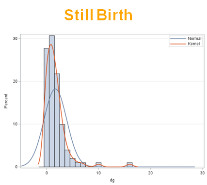
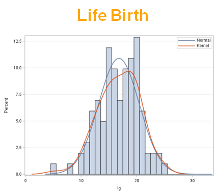
Let’s proceed to the analysis of life and stillbirth. In a previous post, I already showed you how to use the Beta-Binomial to simulate a sample size for these outcomes. Here, I will show you the usability of the Negative-Binomial distribution.
The dataset looks like this in which we have columns for total born, life birth, stillbirth, and mummified. We have this data per sow and per cycle.

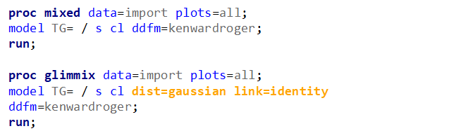
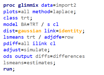
Let's analyze the data using PROC MIXED and PROC GLIMMIX.
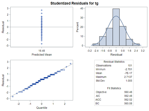
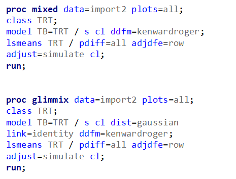
The problem with using a continuous distribution on discrete data is that the results will be presented on a continuum, which results in estimating parts of a piglet.
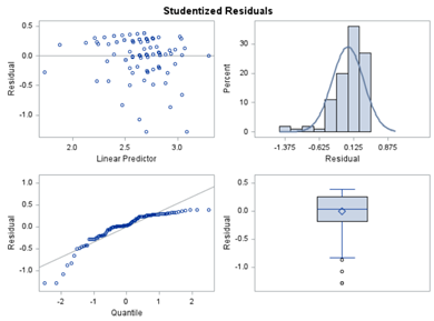
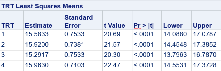
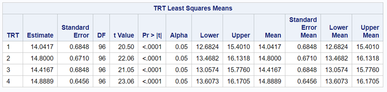
Below, you see the estimates provided via the Normal distribution and the Negative Binomial distribution. Of course, the Normal makes no sense here.

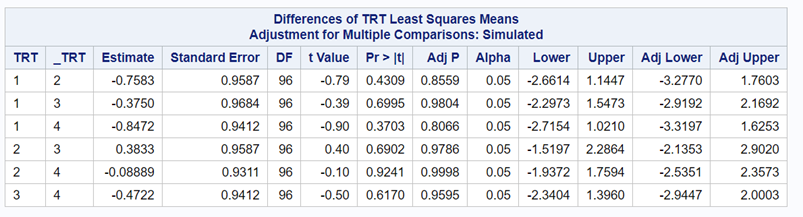

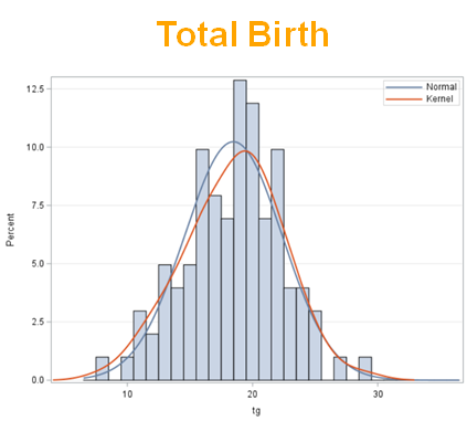
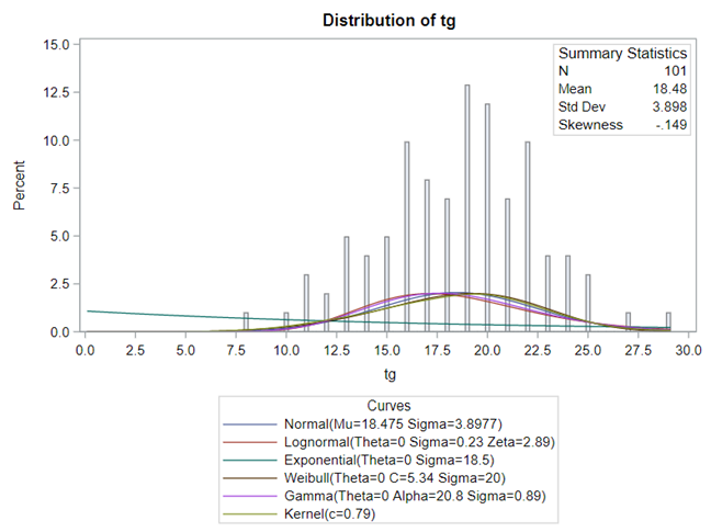
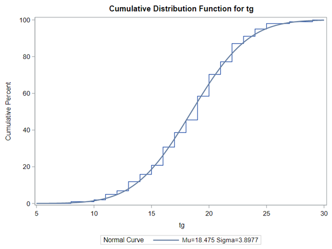
So, analyzing total, still, and life birth in a correct manner is not easy, although it seems very easy. Total birth and life birth seem to follow a normal distribution, but cannot be analyzed as such — how to interpret a treatment gain of 1/5th a piglet?
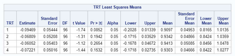
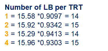
Hence, for total birth and life birth, a Negative Binomial model will do the trick to keep the data in a discrete manner (counts) whilst dealing with the skewness of the variance to the mean. The results will be predicted proportions which you have to multiply to the total to get the predicted integer. Using the Negative Binomial model will increase the standard error of the LSMEANS and LS-Differences by using the correct model.
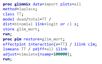
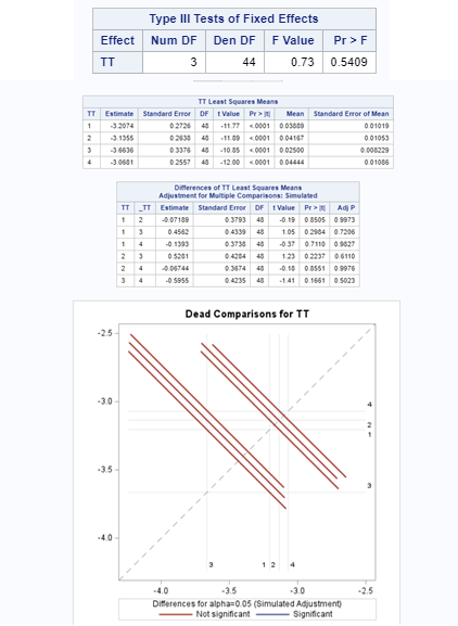
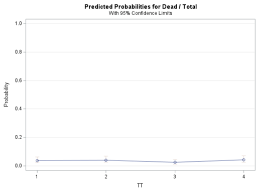
Let's continue with data in which variation is extremely low, such as mortality or footpad lesions. Mortality data in the animal sciences are often difficult to model because they operate at the lower boundary of the scale — luckily.
When dealing with proportions, you can run into problems when there is a complete or quasi-complete separation of values. An example is when you have extreme categories in which treatment 1 shows a 99% ‘Yes’ and treatment 2 a 99% ‘No’. As a result, the treatment completely separates the scores.
This is relatively common in binary/binomial data:
- Every value of the response variable in a given level of the Trt factor is 0 → Probability (Succes | Trt) = 0%
- Every value of the response variable in a given level of the Trt factor is 1 → Probability (Succes | Trt) = 100%
The model will fail to converge → if converged, estimates are not to be trusted and the inference is not valid. Also, maximum likelihood estimation will go to infinity.
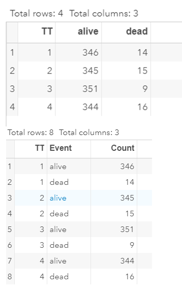
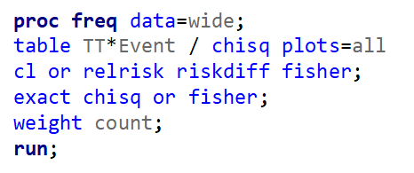
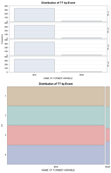
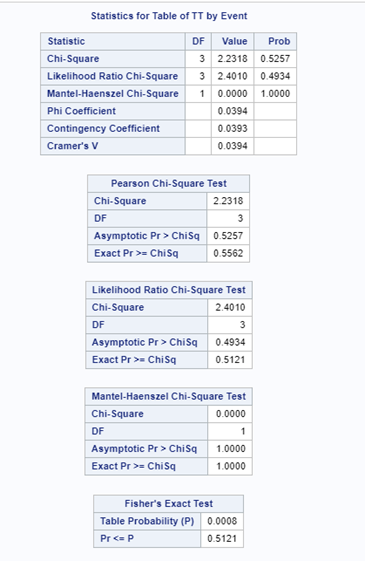
Below is a 2*2 table showing two outcomes for two groups. Comparing these groups can be done via the Odds Ratio, the Relative Risk, the Absolute Risk, and the Risk difference.
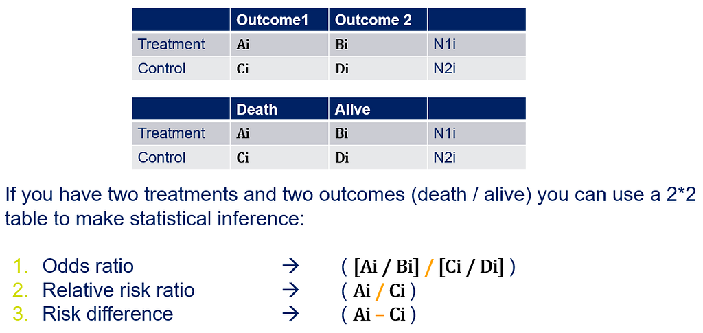
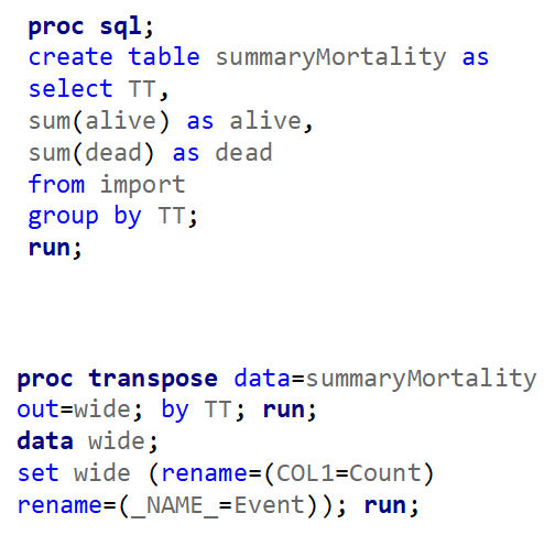
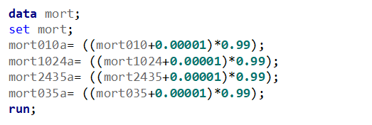
To analyze the mortality data using a 2*2 table, we will need to transform the data.
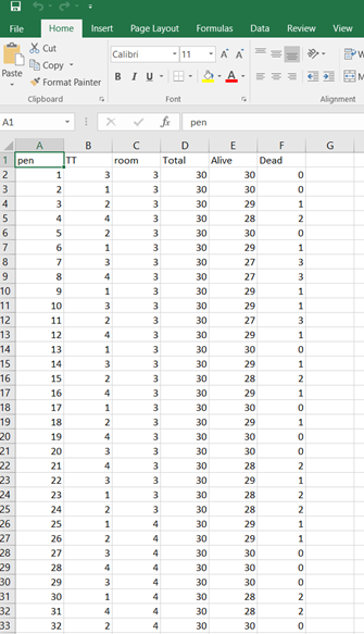
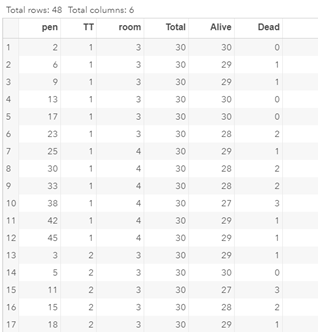
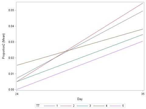
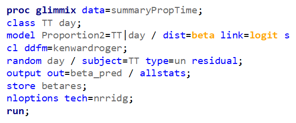
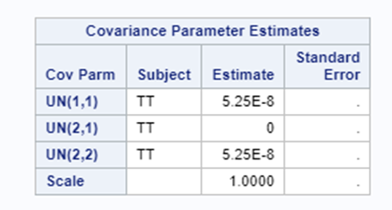

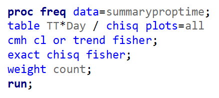
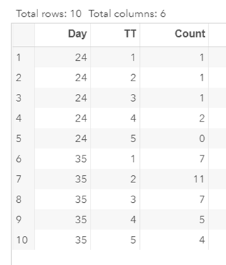

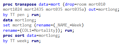
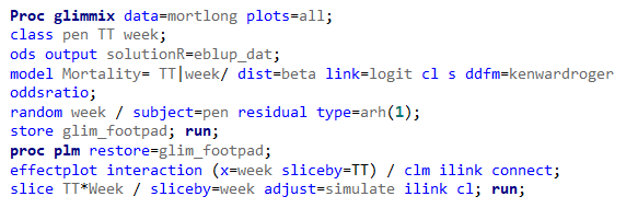
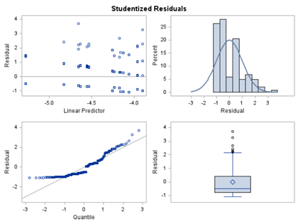
Let's see if can model mortality data using the Beta distribution using another dataset.
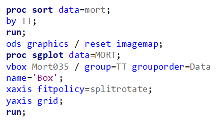
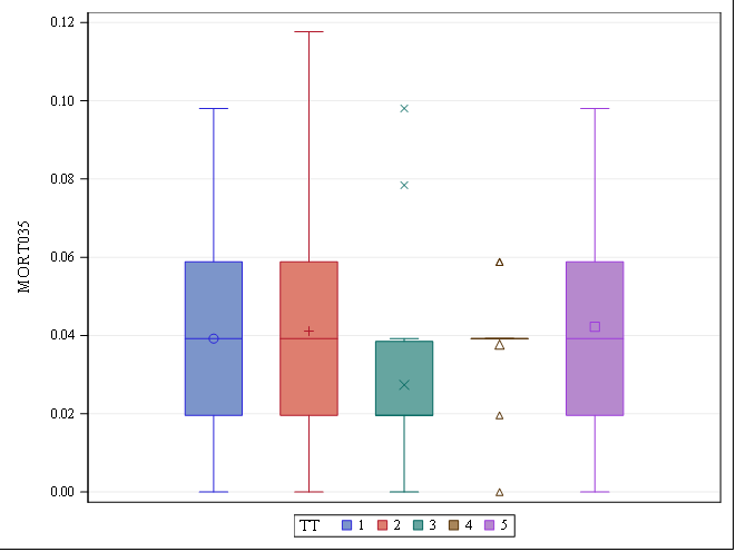

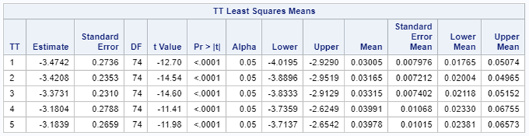
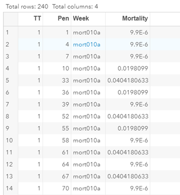
Let's see if we can analyze the mortality data per week.

In summary, data on mortality & footpad lesions are notorious for not having enough variation to analyze. This is because no animal died, and as a result, every animal in every pen gets the same score. In some cases, it is, therefore, best to just use a contingency table to analyze the events. Also, the creation of binary classes and analyzing them as proportions can help get a model from which inferences may be made. However, when there truly is not enough variation, it is best to just report the observed number of events. No statistics!
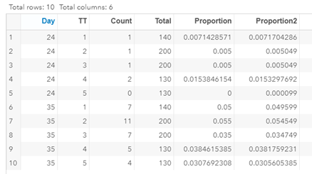
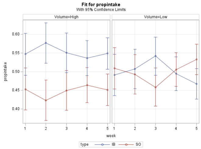
Last, but not least, let's dive into preference studies. Preference studies are quite funny to analyze since they measure the amount of feed eaten by an animal, and split that amount by treatment. Hence, you will have, for each animal, an amount is eaten which can be summarized as a whole by adding up the number of feeds they could choose from. More specifically, if you look at the dataset below, you can see that the total amount eaten is a number that is replicated and that the proportion intake per row is the actual number of interest. However, since we only have two treatments, we are dealing with a zero-sum game. If you know how much is eaten from the first treatment, you also know the other.
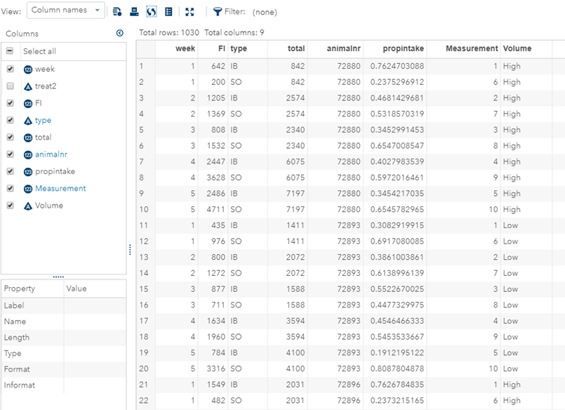
As you can see, per week & per animal, the total feed intake of two products was measured. The design of this experiments and the aggregation of its data makes that the data is dependent:
- Total = 842
- IB = 642
- SO must be 200
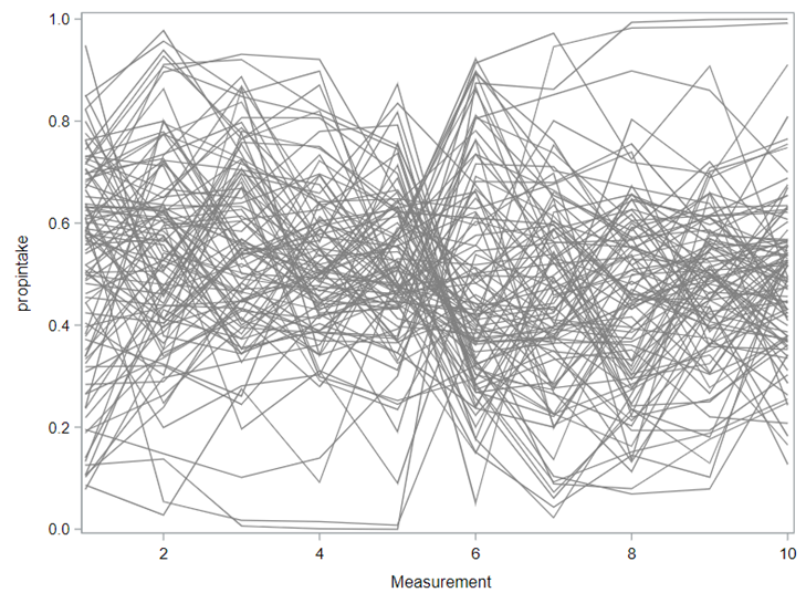
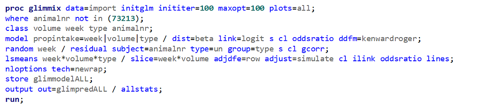
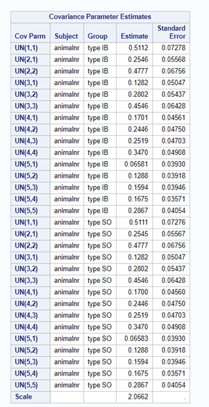
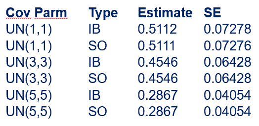
The random week type=un group=type means that I specified a separate unstructured covariance matrix for the IB and SB group. Since the data are mutually exclusive, this makes perfect sense and allows you to use ALL the data.
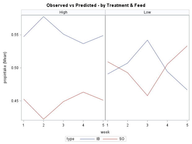
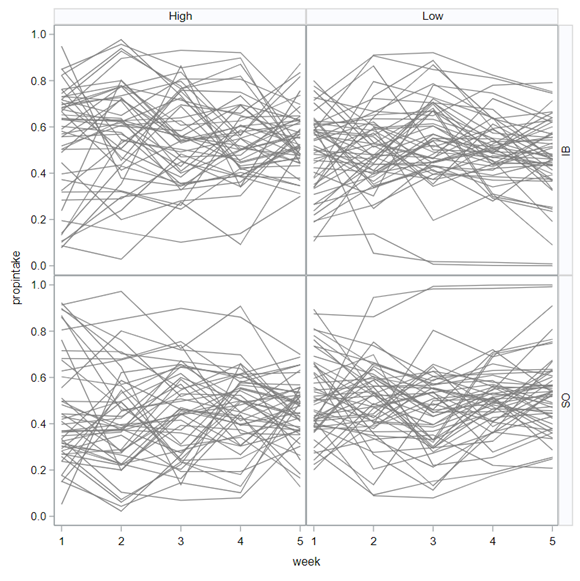
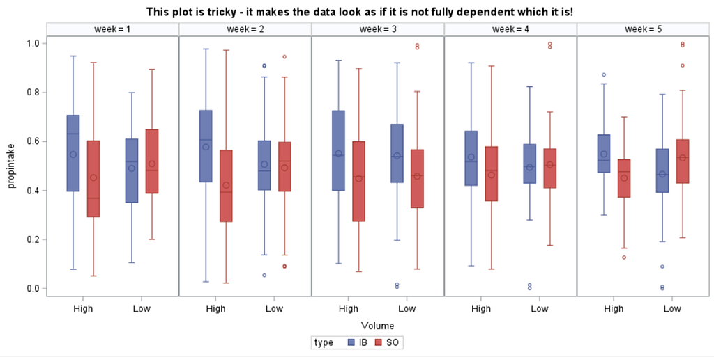
In summary, preference data is by definition dependent data. If you know A-amount ate, you also know B IF you have two treatments. As such, they work like dummy variables. This dependency needs to be included in the mixed model to make it run — random week / residual subject=animalnr type=un group=type. The statement will actually analyze the data double, and so you must compare the results on the raw data with the LSMEANS to make sure you did not make a mistake. Because of the dependency of the data, a mistake is easy to make
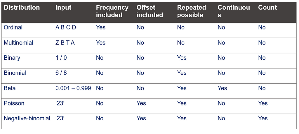
This post marks the end of the PROC GLIMMIX series. Below you can find the last reminder table showing how what each specific distribution needs!
Using PROC GLIMMIX in SAS — examples was originally published in Towards AI on Medium, where people are continuing the conversation by highlighting and responding to this story.
Join thousands of data leaders on the AI newsletter. It’s free, we don’t spam, and we never share your email address. Keep up to date with the latest work in AI. From research to projects and ideas. If you are building an AI startup, an AI-related product, or a service, we invite you to consider becoming a sponsor.
Published via Towards AI
Related posts


Popular posts

 for 2021")


Updates

Recent Posts