Morphable Model Explained

Last Updated on November 25, 2020 by Editorial Team

Author(s): Anton Lebedev 

Morphable 3D models are generative models with an intuitive user interface. Let’s find out how they work and build one

3D modeling is becoming a prominent part of computer science. It is more than 20 years since one of the most noticeable papers — 3D Morphable Face Models was first presented at SIGGRAPH ’99. This paper made a significant long term impact on both applications and subsequent research. In past years, morphable models made a significant advancement in the context of deep learning and were incorporated into many state-of-the-art solutions for face analysis. Nevertheless, the first paper is powerful and scalable enough for building meaningful models for different objects. Let’s find out what the paper was about.

The task was to model faces. The authors presented a technique of creating a generative model with an intuitive user interface. The generative model means the algorithm that generates faces and has some parameters to control the output. The design of the algorithm proposes that these parameters must be simple and understandable by a human.

Can we use this technique for other objects? We can. In Neatsy, we created one for the human foot, and you can try it out on the plot below.

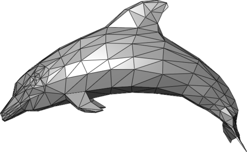
Now, let’s figure out how it works. First of all, we need to understand what a 3D model is. The basic 3D model consists of two components, vertexes (points in the space) and faces (triangles formed by vertexes). Vertexes define the shape of the model’s faces and make the model connected. Vertexes and faces together are called mesh. The more vertexes in the mesh are, the more detailed 3D object results.

In a sense, the 3D model is already parametrized. Every coordinate in every vertex is a parameter we can change, but these changes mostly will make no sense for us because they will break the object structure. So, among all possible ways to change the model, we want to create the most reasonable ones. From this side of view, we need to apply a decomposition on our model. The decomposition task is a classic machine learning task. The problems it solves are dimension reduction and noise reduction. This task has lots of solutions. One of the most popular is PCA.

PCA is a very good choice for us because the task it solves is formulated as: “Find a coordinate system such that the greatest variance by some scalar projection of the data comes to lie on the first coordinate (called the first principal component), the second greatest variance on the second coordinate, and so on.” In other words, PCA finds vectors of the biggest change in data.

Let’s take a look at PCA. PCA takes a matrix with (n, d) shape, where n is the number of objects, d is the number of features. In our case, every object is a scanned foot, and every feature is a vertex coordinate. So the number of features will be 3⋅v, where v is the number of vertexes. The crucial specificity of matrix X is that every column must match a specific point coordinate. For example, all features in a column must be x coordinate of thumb finger edge. So all scans in our dataset must have the same number of points, and these points must be ordered in the same way all over all scans. As a side effect, we obtain the dataset with the same faces overall meshes. Collecting such a dataset for feet is a complex and enjoyable story, but we will skip it for now. If you wish, you can find dataset details for the face model in the original paper.

Now, when we have a dataset, we need to apply PCA to our data. PCA is implemented in many packages. We will use notation in sklearn.decomposition. We are interested in 3 fields.

1. PCA.mean_ — this is a mean foot model. We will use it as a zero point in our morphable model.
2. PCA.componets_ — this is an array of vectors that specify the direction of the greatest change.
3. PCA.explained_variance_ratio_ — This array with importances of every PCA component. Looking at these values, we can decide how many components do we really need in our model.

Now we are ready to create the model. The formula is:

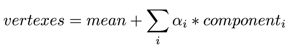
Using the formula above, we make alphas parameters of the model and need to visualize the output. As in our dataset, all faces are the same, we have no need to change them, so we just add them to the resulting mesh.
The result generative model is linear, and at first sight, it shouldn’t be powerful enough to make the components meaningful, but they have a great real-world sense! As you see on the interactive plot, the first parameter is responsible for width, the second is for pronation, and the third is for height. And all these parameters are cruel for describing foot, at least in the case of choosing foot pairs.

And that’s all about building such a model. Now let’s talk about applying it. One of the most impressive ways is to fit this model for real-world objects. As a morphable model describes a 3D object, we can find such parameters of the model that would fit the object on the photo. Then, the fitted model can be used for interpolation of non-visible parts or changing scene and camera parameters.

---

Morphable Model Explained was originally published in Towards AI on Medium, where people are continuing the conversation by highlighting and responding to this story.

Published via Towards AI