Into the Logistic Regression

Last Updated on April 4, 2021 by Editorial Team

Author(s): Satsawat Natakarnkitkul

DATA SCIENCE, MACHINE LEARNING

Break down the concept of logistic regression and one-vs-all and one-vs-one approaches for multi-class classification

Previously I have written in-depths of linear regression both closed-form (equations) and gradient descent. You can read them from the below URL.

Closed-form and Gradient Descent Regression Explained with Python

In this article, I will focus on the Logistic Regression algorithm, break down the concept, think like a machine, and have a look at the concept behind multi-class classifiers using logistic regression.

Linear regression revisited…

Before driving to logistic regression, let’s quickly recap on linear regression.

The linear regression model works well for a regression problem, where the dependent variable is continuous and fails for classification because it treats the classes as numbers (0 and 1) and fits the best hyperplane that minimizes the distances between the points and the hyperplane, hence reduces the error (you can think the hyperplane as model equations for simplicity sake).

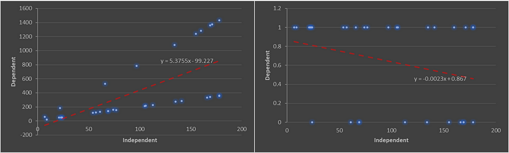
As it can be seen, the prediction of linear regression can go (-∞, ∞). Moreover, it doesn’t give the probabilities as the output.

This is where log-odds come in.

But what are odds and log-odds…

As mentioned earlier, linear regression cannot compute the probability. However, if we looked at probability, it can be easily converted from log-odds, by computing the logarithm of the odds ratio. Probability, odds ratios and log odds are all the same but expressed in different ways.

Probability is the likelihood of an event happens (i.e. 60% chance of students passed the Math exam).

Odds, or odds of success or odds ratio, is a measure of association between an exposure and an outcome, or to simply put, it is the probability of success compared to the probability of failure (from the above example, that’s 0.6/0.4 = 1.5).

Log odds is the logarithm of the odds (ln(1.5) ≅ 0.405).

Remark: in the normal computation, you may use logarithm in any base, but need to be consistent.

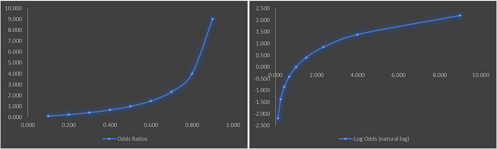
We can visualize the odds ratio against probability and log-odds against the odds ratio. Observe how odds ratio can range [0, ∞), whereas log odds can range between (-∞, ∞).

Now let’s quickly see how we can interpret the odds ratio;

• OR = 1, exposure does not affect odds of the outcome
• OR > 1, exposure associated with higher odds of the outcome
• OR < 1, exposure associated with lower odds of the outcome

Using the above example, the odds of students passed math exams are 1.5 times as large as the odds of students failed math exams. Remember this is not the same as being 1.5 times as probable!

Back to Logistic Regression

I assume that we all know the definition of logistic regression, logistic model (or logit model) is the statistical method to model the probability of a certain class or event (i.e. students passing the exam, customer churn). In this model, we assume a linear relationship between the independent variables and the log-odds for the dependent variable, which can then represent as below equation.

The function that converts log-odds to probability is the logistic function and the unit of measurement for the log-odds scale is called logit, which is from logistic unit (hence, the name).

So from the equation above, ultimately, we try to predict the left path of the equation (not the right) because p(y=1|x) is what we want. So we can take the inverse of this logit function, then we will get something similar to us.

The above equation is the common sigmoid function, logistic sigmoid, which returns the class probability of p(y=1|x) from the inputs b0 + b1x1 + …

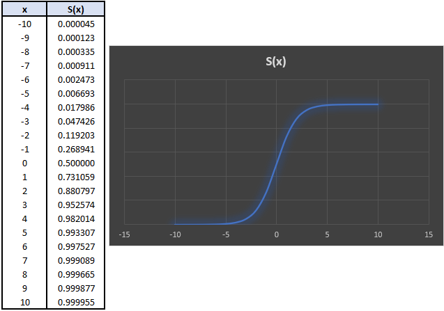
As the logistic curve implied in the y-axis, this mapping is probabilities (0, 1). Ultimately, the reason we use the logarithm of an odds is it can take any positive or negative value (as previously plotted). Hence, logistic regression is a linear model for the log-odds.

Note that in the logistic equation, the parameters are chosen to maximize the likelihood of observing the sample values (or MLE — Maximize Likelihood Estimation) instead of minimizing the sum of squared errors (or LSE — Least Square Estimation).

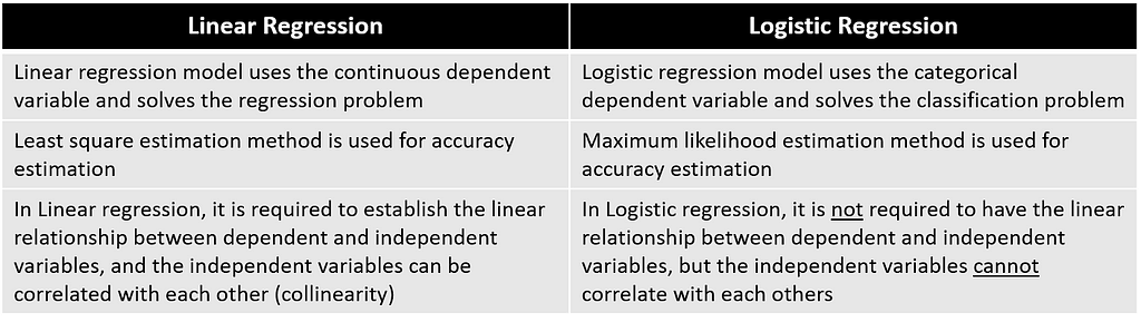
Recap: comparison between linear and logistic regression

What if we have more than two classes to predict…

What I have discussed so far is only for binary logistic regression (dependent variable consists of only two classes — yes or no, 0 or 1). In this section, we will go through multinomial logistic regression, or we may know it as multi-class logistic regression.

To break this down, we already have a binary classification model (logistic regression), eventually, we can split the multi-class dataset into multiple binary classification datasets and fit the model to each.

How does it work then …

Well.. have you ever in a situation where you need to make a guess (let’s imagine in the examination — multiple choices exam). You read the question, compare the choice, cut out the non-sense, compare the remaining choices and pick one.

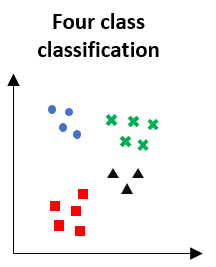
Actually, this can be applied to how the binary classification model works against multi-class problems. So it depends on how you make the comparison, assuming we have four classes: A, B, C, and D. You may choose to compare by A vs. [B, C, D] or compare A to each individual class (i.e. A vs B, A vs C). These two comparisons actually have names and they are One-vs-All and One-vs-One strategies.

One-vs-All Strategy

One-vs-All, OvA (or One-vs-Rest, OvR) is one of the strategies for using binary classification algorithms for multi-class classification.

In this approach, we will focus on one class as a positive class and the other classes are assumed to be a negative class (think of comparing one against the rest of the classes).

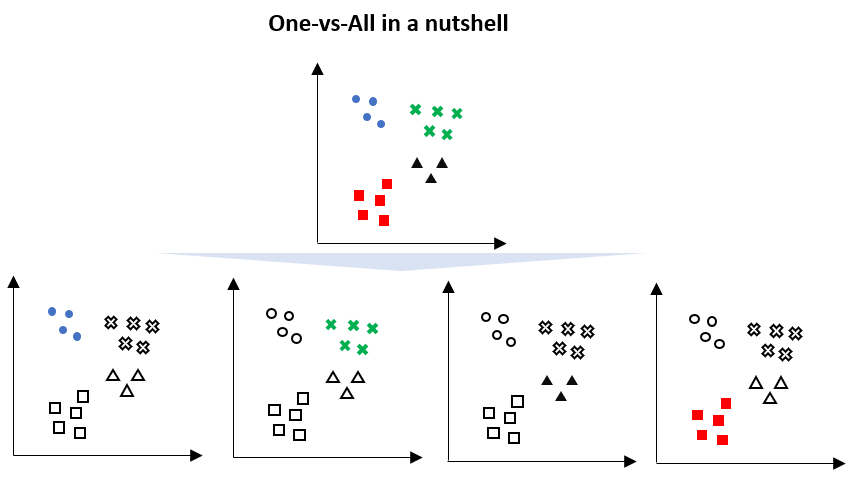
For example, given a multi-class problem with four classes (as per the above visualization), then we can divide these into four binary classification datasets;

• 1: blue vs [green, black, red]
• 2: green vs [blue, black, red]
• 3: black vs [blue, green, red]
• 4: red vs [blue, green, black]

This strategy requires that each model predicts a probability-like score. The argmax of these scores is then used to predict a class. This strategy is normally used for algorithms such as;

1. Logistic regression
2. Perception
3. Deep neural network with softmax function as an output layer

As such, the scikit-learn library implements the OvA / OvR by default when using these algorithms to solve multi-class problems.

A couple of possible downsides of this approach is when it handles very large datasets.

One-vs-One strategy

Similar to the One-vs-All strategy, the one-vs-one strategy is a method for binary classification for multi-class problems by splitting the dataset into binary classification datasets. Unlike the one-vs-all strategy, one-vs-one splits the dataset onto two specific classes, an example is illustrated below.

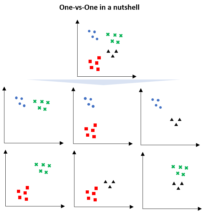
Because of this split, there are more binary classification models than one-vs-all strategy;

1. blue vs green
2. blue vs red
3. blue vs black
4. red vs green
5. red vs black
6. green vs black

The number of models generated = (n_classes * (n_classes -1))/2

Once all the models are generated, the point will be tested to all models and recorded how many times a class is preferred with the other classes. The class having the majority of votes wins.

Normally, this strategy is suggested for support vector machines and related kernel-based algorithms because the performance of the kernel method does not scale in proportion to the size of the training dataset, and using only subsets of the training data may counter this effect.

So which strategy is better?

As outlined above, a one-vs-all strategy can be challenging to deal with large datasets as we still use all of the data multiple times. However, the one-vs-one strategy splits the full dataset into a binary classification for each pair of classes (see the visualization on OvA and OvO above).

The one-vs-all strategy trains a fewer number of classifiers, making it a faster option. However, the one-vs-one strategy is less prone to create an imbalance in the dataset.

Conclusion

In this article, I have a walkthrough;

• review the linear regression;
• the basic concept of log-odds and why it is being used;
• deeper dive into the concept of logistic regression;
• one-vs-all and one-vs-one strategy for the multi-class classifier.

Hopefully, you gain more knowledge and the background of logistic regression to extend your thoughts and build upon those (instead of just importing the logistic regression library/package and use it).

Reference and External Links

• 4.2 Logistic Regression | Interpretable Machine Learning
• Logistic regression – Wikipedia
• sklearn.multiclass.OneVsRestClassifier – scikit-learn 0.24.1 documentation
• sklearn.multiclass.OneVsOneClassifier – scikit-learn 0.24.1 documentation

---

Into the Logistic Regression was originally published in Towards AI on Medium, where people are continuing the conversation by highlighting and responding to this story.

Published via Towards AI