SUPPORT VECTOR MACHINES : PREDICTING FUTURE – CASE STUDY

Author(s): Data Science meets Cyber Security

Originally published on Towards AI the World’s Leading AI and Technology News and Media Company. If you are building an AI-related product or service, we invite you to consider becoming an AI sponsor. At Towards AI, we help scale AI and technology startups. Let us help you unleash your technology to the masses.

SUPPORT VECTOR MACHINES: PREDICTING FUTURE – CASE STUDY

CONTINUATION OF SUPERVISED LEARNING METHODS: PART-3

As previously promised in SUPPORT VECTOR MACHINE — 3RD PART OF SUPERVISED LEARNING METHODS, let’s talk about an amazing case study to analyze and comprehend the application of support vector into a real business problem and be ready for the amazing outcomes and prediction no one actually saw coming.

PROBLEM STATEMENT :

In this problem statement, we’ll study the case where we’ll try to predict whether the person will survive based on the diagnostic factors influencing Hepatitis.

Let’s first talk about the dataset we are going to use. The dataset contains the occurrences of hepatitis in people.

WHAT ABOUT THE SOURCE OF THIS DATASET?

The UCI machine learning repository was used to get this data set.. It has 155 recordings in two separate types, 32 of which are death records and 123 of which are live records. There are 20 characteristics in the dataset (14 binary and 6 numerical attributes)

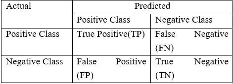
We’ll use a number of methods in this case study to successfully predict whether the person will survive or not based on the diagnostic factors influencing Hepatitis on the right error metrics. One of these methods would be the CONFUSION MATRIX.

If you are unclear about this pitch, please refer to our prior blog post on confusion metrics. (Comes under the blog WORLD OF CLASSIFICATION)

LET’S BEGIN WITH THE PRACTICAL PART:

STEP1: LOADING THE REQUIRED AND MANDATORY LIBRARIES:

#THIS WILL HELP US IGNORE THE WARNINGS WHILE RUNNING OUR CODE
import warnings
warnings.filterwarnings("ignore")

import os
import numpy as np
import pandas as pd
 
from sklearn.model_selection import train_test_split
from sklearn.preprocessing import StandardScaler, OneHotEncoder
 
from sklearn.impute import SimpleImputer
 
from sklearn.svm import SVC
 
from sklearn.metrics import confusion_matrix, accuracy_score, recall_score, precision_score, f1_score
 
from sklearn.model_selection import GridSearchCV

STEP2: READING THE HEPATITIS DATASET:

data = pd.read_csv("/content/hepatitis.csv")

EXPLORATORY DATA ANALYSIS:

IMPORTANCE: An EDA is a detailed analysis designed to reveal a data set’s underlying structure. It is significant for a business problem because it reveals trends, patterns, and linkages that are not immediately obvious.

#Checking the dimensions (rows and columns)
data.shape

#Checking the datatypes of each variable
data.dtypes

#Checking the head of the data (i.e top 5 rows)
data.head()

#Checking the basic summary statistics
data.describe()
#Checking the number of unique levels in each attribute
data.nunique()

#Target attribute Distribution
data.target.value_counts()

data.target.value_counts(normalize=True)*100

STEP3: DATA PRE-PROCESSING:

WHY WE NEED TO PRE-PROCESS DATA EXACTLY?

Every time we decide to work with data, the first step is to gather the data, which is typically in the unclassified and uncleaned form. Once we start working with this data, it becomes very challenging for the data scientist to find clear patterns and outcomes through that type of data, which can result in many false positives and negatives as well as confusion.

So, in order to prevent this kind of a mess, we clean and preprocess the raw data to increase accuracy and dependability. We also eliminate missing (i.e., null spaces within the data) or inconsistent data values to allow algorithms or models to run smoothly without experiencing any significant error values.

In order to make the raw data more comprehensible, practical, and effective, data pre-processing is also regarded as a crucial method employed in data mining. This entire data pre-processing procedure aids in improving our outcomes.

#Let's drop the columns which are not that signicant and in use
data.drop(["ID"], axis = 1, inplace=True)

#Storing categorical and numerical values:
num_cols = ["age", "bili", "alk", "sgot", "albu", "protime"]

cat_cols = ['gender', 'steroid', 'antivirals', 'fatigue', 'malaise', 'anorexia', 'liverBig',
           'liverFirm', 'spleen', 'spiders', 'ascites', 'varices', 'histology']

#Checking the head of dataset once again to see how dataframe looks
data.head()

#Converting the attributes into appropriate type to avoid the future error
data[cat_cols] = data[cat_cols].astype('category')

#After converting the attribute types check the datatypes to be sure once again
data.dtypes

STEP4: SPLITTING DATA INTO ‘X’ AND ‘Y’:

#Time to split the data into X and Y
X = data.drop(["target"], axis = 1)
y = data["target"]

#Getting the shape of data
print(X.shape, y.shape)

#Training the data
X_train, X_test, y_train, y_test = train_test_split(X, y, test_size = 0.2, random_state = 123, stratify=y)

#Getting the shape of trained data to find the difference between untrained and trained data.
print(X_train.shape)
print(X_test.shape)
print(y_train.shape)
print(y_test.shape)

#Check for distribution target variables
y_train.value_counts()

y_train.value_counts(normalize=True)*100

STEP5: DATA PRE-PROCESSING AFTER SPLITTING THE DATA INTO ‘X’ AND ‘Y’:

#Checking the null values
X_train.isna().sum()

X_test.isna().sum()

IMPUTATION MISSING CATEGORICAL COLUMNS WITH MODE:

df_cat_train = X_train[cat_cols]
df_cat_test = X_test[cat_cols]

cat_imputer = SimpleImputer(strategy='most_frequent')
cat_imputer.fit(df_cat_train)

df_cat_train = pd.DataFrame(cat_imputer.transform(df_cat_train), columns=cat_cols)
df_cat_test = pd.DataFrame(cat_imputer.transform(df_cat_test), columns=cat_cols)

df_num_train = X_train[num_cols]
df_num_test = X_test[num_cols]

IMPUTATION OF MISSING NUMERICAL COLUMNS WITH MEDIAN:

num_imputer = SimpleImputer(strategy='median')
num_imputer.fit(df_num_train[num_cols])

df_num_train = pd.DataFrame(num_imputer.transform(df_num_train), columns=num_cols)
df_num_test =  pd.DataFrame(num_imputer.transform(df_num_test), columns=num_cols)

NOW, COMBINING THE IMPUTED CATEGORICAL AND NUMERIC COLUMNS:

# Combine numeric and categorical in train
X_train = pd.concat([df_num_train, df_cat_train], axis = 1)
 
# Combine numeric and categorical in test
X_test = pd.concat([df_num_test, df_cat_test], axis = 1)

STANDARDISING THE NUMERICAL ATTRIBUTES:

​​Since the method we are employing makes assumptions about the various forms of distribution, such as linear and logistic regression, standardization is a highly helpful strategy that aids us when our data has diverse scales.

When a regression model uses variables that are expressed as polynomials or interactions, data scientists often standardize the data for that model. Due to the terms’ significant importance and ability to reveal the connection between the response and predictor factors, they can also result in extremely high levels of multicollinearity.

scaler = StandardScaler()
scaler.fit(X_train[num_cols])

X_train_std = scaler.transform(X_train[num_cols])
X_test_std = scaler.transform(X_test[num_cols])

print(X_train_std.shape)
print(X_test_std.shape)

ONEHOTENCODER: CONVERTING CATEGORICAL ATTRIBUTES TO NUMERIC ATTRIBUTES:

WHY?

All input and output variables for machine learning models must be numeric. This means that in order to fit and assess a model, categorical data must first be encoded to numbers in your data.

enc = OneHotEncoder(drop = 'first')
enc.fit(X_train[cat_cols])

X_train_ohe=enc.transform(X_train[cat_cols]).toarray()
X_test_ohe=enc.transform(X_test[cat_cols]).toarray()

CONCATENATE ATTRIBUTE:

Standardised numerical attributes and categorical attributes with one-hot encoding.

X_train_con = np.concatenate([X_train_std, X_train_ohe], axis=1)
X_test_con = np.concatenate([X_test_std, X_test_ohe], axis=1)

print(X_train_con.shape)
print(X_test_con.shape)

STEP6: FINALLY BUILDING MODEL SUING LINEAR SVM:

CREATING A SVC CLASSIFIER USING A LINEAR KERNEL:

linear_svm = SVC(kernel='linear', C=1)

#Training the classifier
linear_svm.fit(X=X_train, y= y_train)

#Predicting the results
train_predictions = linear_svm.predict(X_train)
test_predictions = linear_svm.predict(X_test)

ERROR MATRIX:

An evaluation procedure that aids in determining and forecasting the viability of a classification model is known as a confusion matrix, also known as an error matrix. You can observe the many prediction mistakes you could make by using confusion matrices.

#Defining the error matrix
def evaluate_model(act, pred):
   print("Confusion Matrix \n", confusion_matrix(act, pred))
   print("Accuracy : ", accuracy_score(act, pred))
   print("Recall   : ", recall_score(act, pred))
   print("Precision: ", precision_score(act, pred))
   print("F1_score : ", f1_score(act, pred))

### Train data accuracy
evaluate_model(y_train, train_predictions)
 
### Test data accuracy
evaluate_model(y_test, test_predictions)

As much as I liked writing for you guys, I hope you enjoyed implementing and learning from this case study as well. If you have any questions or need assistance with the dataset source or GitHub gist (if you are having trouble with parts of the code), please get in touch; we would be more than happy to assist.😁❤️

CONTINUE TO FORESEE, LEARN, AND EXPLORE! ❤️

FOLLOW US FOR THE SAME FUN TO LEARN DATA SCIENCE BLOGS AND ARTICLES:💙

LINKEDIN: https://www.linkedin.com/company/dsmcs/

INSTAGRAM: https://www.instagram.com/datasciencemeetscybersecurity/?hl=en

GITHUB: https://github.com/Vidhi1290

TWITTER: https://twitter.com/VidhiWaghela

MEDIUM: https://medium.com/@datasciencemeetscybersecurity-

WEBSITE: https://www.datasciencemeetscybersecurity.com/

– TEAM DATA SCIENCE MEETS CYBER SECURITY ❤️💙

---

SUPPORT VECTOR MACHINES : PREDICTING FUTURE – CASE STUDY was originally published in Towards AI on Medium, where people are continuing the conversation by highlighting and responding to this story.

Join thousands of data leaders on the AI newsletter. It’s free, we don’t spam, and we never share your email address. Keep up to date with the latest work in AI. From research to projects and ideas. If you are building an AI startup, an AI-related product, or a service, we invite you to consider becoming a sponsor.

Published via Towards AI