Learn with me: Linear Algebra for Data Science — Part 3: Eigenvectors

Author(s): Matthew Macias

Originally published on Towards AI the World’s Leading AI and Technology News and Media Company. If you are building an AI-related product or service, we invite you to consider becoming an AI sponsor. At Towards AI, we help scale AI and technology startups. Let us help you unleash your technology to the masses.

Learn With Me: Linear Algebra for Data Science — Part 3: Eigenvectors

I know what you are thinking, what on earth is an eigenvector? Is that even an actual word?

Yes, they are real. They are also extremely helpful for certain operations in Data Science. If you read Part 2 of this series, you’ll know that I encouraged you to start to think of matrices as a means to perform linear transformations. A common way to think about this is through the classic Ax = b example, where matrix A transforms the input vector x into the output vector b.

So, what is an Eigenvector?

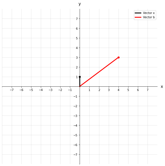
An eigenvector is probably best explained through an example. Let’s start with a matrix A and a vector x:

For those of you who have read the earlier parts of this series, the above dot product will be a piece of cake! The matrix A transforms vector x into a new vector b which has a value of [4, 3] . Let’s see this transformation visually.

We could describe this transformation as a rotating and stretching of the original vector x. We can go one step further and visualize a field of vectors represented by a circle. Imagine that each point that lies on this circle is the tip of a vector that originates at the origin. Now we can see how all different vectors would transform as a result of matrix A.

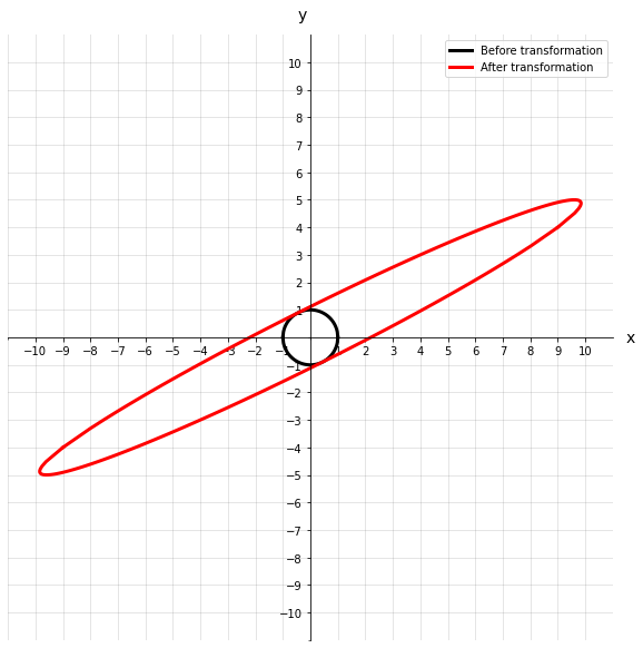
As you can see, the original circle gets rotated and stretched out quite a bit. If we imagine those points along the circle as vectors, then the same would be said for them. But what if there was a vector that wasn’t rotated during the transformation? How would we find it? And better yet, why should we care about it?

Well, that’s exactly what an eigenvector is, a vector that is not rotated during a linear transformation, only scaled. Formally we can denote it as:

Where λ (lambda) is referred to as an eigenvalue. It’s just a scalar that tells us by how much the eigenvector was shortened or lengthened after the linear transformation. A matrix may have some eigenvalues or none (for a matrix to have any eigenvectors, to begin with, it must be a square matrix), but each one of those eigenvectors has a corresponding eigenvalue that tells us about the scaling.

Continuing our example above, let’s see what an eigenvector and eigenvalue of matrix A look like.

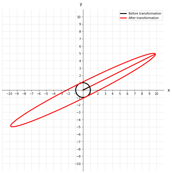
We can see that before and after the transformation, the eigenvector does not rotate off its original axis. This eigenvector also has an eigenvalue of 11, which intuitively makes sense because the vector after transformation looks about 11 times longer.

Calculating Eigenvectors

If all you want to know is what Python code to execute to return both the eigenvalues and eigenvectors, here you are:

eig_vals, eig_vecs = np.linalg.eig(A)

For the more curious among you, we will go through how you might derive the eigenvalues and vectors manually. I will preface the math by saying you will probably never do this for practical reasons, but it’s really good to get an understanding of what is going on under the hood of the NumPy functions.

Let’s go back to our original math form of eigenvectors and eigenvalues.

The first thing we will do is add an identity matrix into the mix. These matrices don’t change anything (they are the equivalent of multiplying a number by 1), but they simplify the calculation. Our new equation becomes:

Let’s bring everything to one side because having things equal to zero makes it exciting! We will also factor out an x as that will be a commonality.

For now, we will just take for granted that the terms within the brackets result in a matrix that is not invertible. At this point, it doesn’t seem like there are many other options. However, the fact that the resulting matrix is not invertible tells us something pretty important. The determinant of the terms within the brackets must also equal 0. That is:

Next, we will calculate the matrix within the brackets using our original A matrix:

Once we have that matrix, we can go about solving for its determinant. For a 2×2 matrix that is relatively simple, I would not recommend trying this manually for any larger matrices. In this case, it’s just the (top left * bottom right) — (bottom left * top right). This results in an equation that we can factorize to find our eigenvalues:

So far, it all looks good, we are getting the same eigenvalues as we did with Python. But the work is not done, we need to use our eigenvalues to calculate our eigenvectors. Using what we have defined so far, let's fill in the standard equation for eigenvectors:

We actually have an eigenvalue now that we can use as input into the above equation. Using 11, we will get a system of equations like the below:

These are pretty straightforward equations, and they are both solved by:

So any set of points that satisfy the above criteria will lie on our eigenvector. There you have it, you’ve just calculated the eigenvalues and eigenvectors for matrix A. But, there is still one major question looming…

Who cares?

What was the point of all of this? I hear you say. Well, believe it or not, this does have its place in Data Science. We will briefly discuss one major application of eigenvalues and eigenvectors.

Principal Components Analysis (PCA)

You may or may not have heard of principal components analysis. It is perhaps the most used dimensionality reduction technique in Data Science. It serves to reduce the amount of data required to represent a system whilst also maintaining as much information as possible. PCA effectively takes the eigenvectors of the covariance matrix and returns what is known as principal components. We will cover PCA more in-depth in later parts of the series, but for now, just know how important it is!

Conclusion

Hopefully, you enjoyed another part of the linear algebra series, be sure to check out Part 1 and Part 2 if there was anything you were unsure about going through this article. We have laid a pretty nice foundation up to this point, and we will start to get into more practical applications of linear algebra, such as PCA and singular value decomposition (SVD).

---

Learn with me: Linear Algebra for Data Science — Part 3: Eigenvectors was originally published in Towards AI on Medium, where people are continuing the conversation by highlighting and responding to this story.

Join thousands of data leaders on the AI newsletter. It’s free, we don’t spam, and we never share your email address. Keep up to date with the latest work in AI. From research to projects and ideas. If you are building an AI startup, an AI-related product, or a service, we invite you to consider becoming a sponsor.

Published via Towards AI