Text Classification with RNN

Last Updated on November 21, 2020 by Editorial Team

Author(s): Aarya Brahmane

 

Deep Learning

Recurrent Neural Networks, a.k.a. RNN is a famous supervised Deep Learning methodology. Other commonly used Deep Learning neural networks are Convolutional Neural Networks and Artificial Neural Networks. The main goal behind Deep Learning is to reiterate the functioning of a brain by a machine. As a result of which, loosely, each neural network structure epitomizes a part of the brain.

Artificial Neural Network, a.k.a. ANN stores data for a long time, so does the Temporal lobe. So it is linked with the Temporal Lobe. Convolutional Neural Networks, a.k.a. CNN, are used in image classification and Computer Vision tasks. The same work in our brain is done by Occipital Lobe and so CNN can be referenced with Occipital Lobe. Now, RNN is mainly used for time series analysis and where we have to work with a sequence of data. In such work, the network learns from what it has just observed, i.e., Short-term memory. As a result of which, it resembles the Frontal Lobe of the brain.

Importing Data

In this article, we will work on Text Classification using the IMDB movie review dataset. This dataset has 50k reviews of different movies. It is a benchmark dataset used in text-classification to train and test the Machine Learning and Deep Learning model. We will create a model to predict if the movie review is positive or negative. It is a binary classification problem. This dataset can be imported directly by using Tensorflow or can be downloaded from Kaggle.

from tensorflow.keras.datasets import imdb

Preprocessing the Data

The reviews of a movie are not uniform. Some reviews may consist of 4–5 words. Some may consist of 17–18 words. But while we feed the data to our neural network, we need to have uniform data. So we pad the data. There are two steps we need to follow before passing the data into a neural network: embedding and Padding. In the Embedding process, words are represented using vectors. The position of a word in a vector space is learned from the text, and it learns more from the words it is surrounded by. The embedding layer in Keras needs a uniform input, so we pad the data by defining a uniform length.

sentence=['Fast cars are good',
          'Football is a famous sport',
          'Be happy Be positive']

After padding:

[[364  50  95 313   0   0   0   0   0   0]  
 [527 723 350 333 722   0   0   0   0   0]  
 [238 216 238 775   0   0   0   0   0   0]]

In the above snippet, each sentence was padded with zeros. The length of each sentence to input is 10, and so each sentence is padded with zeroes. You can find the complete code for word embedding and padding at my GitHub profile.

Building an RNN model

Recurrent Neural Networks work in three stages. In the first stage, it moves forward through the hidden layer and makes a prediction. In the second stage, it compares its prediction with the true value using the loss function. Loss function showcases how well a model is performing. The lower the value of the loss function, the better is the model. In the final stage, it uses the error values in back-propagation, which further calculates the gradient for each point (node). The gradient is the value used to adjust the weights of the network at each point.

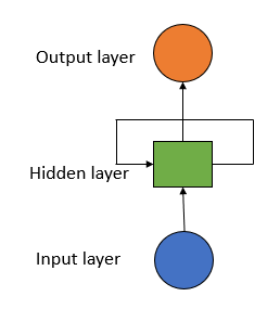
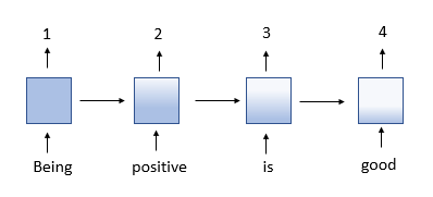
Recurrent Neural Networks are commonly used when we are dealing with sequential data. The reason is, the model uses layers that give the model a short-term memory. Using this memory, it can predict the next data more accurately. The time for which the information about the past data will be kept is not fixed, but it depends on the weights allotted to it. Thus, RNN is used in Sentiment Analysis, Sequence Labeling, Speech tagging, etc.

The first layer of the model is the Embedding Layer:

# Embedding Layer

imdb_model.add(tf.keras.layers.Embedding(word_size, embed_size, input_shape=(x_train.shape[1],)))

The first argument of the embedding layer is the number of distinct words in the dataset. This argument is defined as large enough so that every word in the corpus can be encoded uniquely. In this project, we have defined the word_size to be 20000. The second argument shows the number of embedding vectors. Each word in the corpus will be shown by the size of the embedding.

The second layer of the model is LSTM Layer:

# LSTM Layer

imdb_model.add(tf.keras.layers.LSTM(units=128, activation='tanh'))

This is by far the most important concept of a Recurrent Neural Network. LSTM- Long Short Term Memory layer solves the problem of Vanishing gradient and thus gives the model the memory to predict the next word using recent past memory.

Vanishing Gradients:

As mentioned before, the Gradient is the value used to adjust the weight at each point. The bigger is the gradient. The bigger is the adjustment and vice versa. Now the problem is, in backpropagation, each node in the layer calculates its gradient value from the gradient value of the previous layer.

So if the gradient value of the previous layer was small, the gradient value at that node would be smaller and vice versa. And so, going down the stream of backpropagation, the value of the gradient becomes significantly smaller. Since the gradients are very small, near to null. The weight at each point is barely adjusted, and thus their learning is minimum. With minimum learning, the model fails to understand the contextual data.

Wrec: Recorded weight at each point

Wrec < 1: Vanishing Gradient   
Wrec > 1: Exploding Gradient

The solution to this problem was proposed by Hochreiter & Schmidhuber in 1997. It was LSTM. Long-Short Term Memory would control the flow of data in the backpropagation. The internal mechanism has gates in them, which calculate the flow of information, and prevents weight to get decreased beyond a certain value. By stacking the model with the LSTM layer, a model becomes deeper, and the success of a deep learning model lies in the depth of the model.

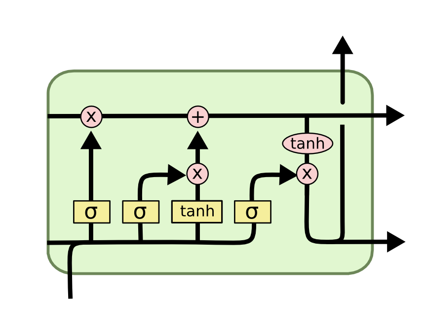
In LSTM, the gates in the internal structure pass only the relevant information and discard the irrelevant information, and thus going down the sequence, it predicts the sequence correctly. For detailed information on the working of LSTM, do go through the article of Christopher Olah.

Activation Function

In the RNN model activation function of “Hyperbolic tangent(tanh(x))” is used because it keeps the value between -1 to 1. During backpropagation, the weights at node get multiplied by gradients to get adjusted. If the gradient value is more, the weight value will increase a lot for that particular node. As a result of which, the weights of other nodes will be minimum and would not count towards the learning process. This, in turn, will lead to a high bias in the model. So to avoid this, tanh(z) hyperbolic function is used. It brings the values between -1 to 1 and keeps a uniform distribution among the weights of the network.

tanh(z) = [exp(z) - exp(-z)] / [exp(z) + exp(-z)]

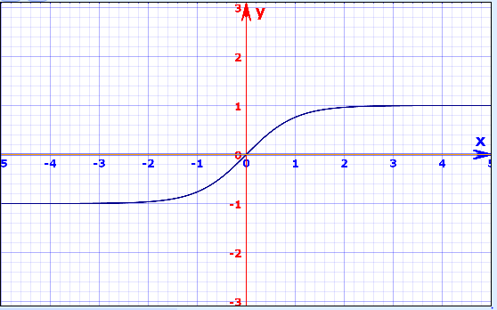
The other advantage of a hyperbolic tangent activation function is that the function converges faster than the other function, and also the computation is less expensive.

# Output Layer

imdb_model.add(tf.keras.layers.Dense(units=1, activation='sigmoid'))

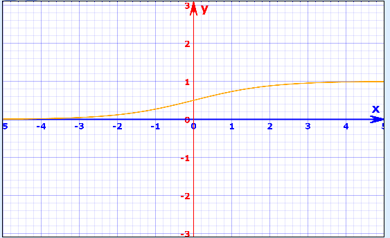
In the output layer, the “Sigmoid” activation function is used. Like “Hyperbolic Tangent,” it also shrinks the value, but it does it between 0 to 1. The reasoning behind this is, if a value is multiplied by 0, it will be zero and can be discarded. If a value is multiplied by 1, it will remain zero and will be here only. Thus by using the sigmoid function, only the relevant and important value will be used in predictions.

Compiling the layers:

imdb_model.compile(optimizer='rmsprop', loss='binary_crossentropy', metrics=['accuracy'])

In this text classification problem, we are predicting a positive review or a negative review. Thus we are working on a binary classification problem. So we use the loss function of “binary_crossentropy.” Also, the metrics used will be “accuracy.” When we are dealing with a multi-class classification problem, we use “sparse-categorical cross-entropy” and “sparse accuracy.” Multi-class classification problems mainly use CNN. For more information, you can read my article on CNN.

While training the model, we train the model in batches. Instead of training a single review at a time, we divide it into batches. This reduces the computational power. We have used a batch size of 128 for the model.

imdb_model.fit(x_train, y_train, epochs=5, batch_size=128)

You can improvise the model by changing epochs and batch_size. But do keep a look at overfitting too! By using this model, I got an accuracy of nearly 84%.

So, in this article, we understood what Recurrent Neural Networks are. We went through the importance of pre-processing and how it is done in an RNN structure. We learned about the problem of Vanishing Gradient and how to solve it using LSTM. Finally, we read about the activation functions and how they work in an RNN model.

You can find the complete code of this model on my GitHub profile.

Feel free to connect with me at https://www.linkedin.com/in/aarya-brahmane-4b6986128/

References:

This is a great article to get a deeper understanding of LSTM with great visual representation https://colah.github.io/posts/2015-08-Understanding-LSTMs/

One can find and make some interesting graphs at https://www.mathsisfun.com/data/function-grapher.php#functions

Happy Deep Learning!

Peace!

---

Text Classification with RNN was originally published in Towards AI on Medium, where people are continuing the conversation by highlighting and responding to this story.

Published via Towards AI